Binary Classification Neural Network from Scratch

Packages

We first import necessary packages:

• numpy is the main package for scientific computing with Python.
• matplotlib is a library to plot graphs in Python.
• h5py is a Pythonic interface to the HDF5 binary data format.

import numpy as np
import h5py
import matplotlib.pyplot as plt

%matplotlib inline
plt.rcParams['figure.figsize'] = (5.0, 4.0) # set default size of plots
plt.rcParams['image.interpolation'] = 'nearest'
plt.rcParams['image.cmap'] = 'gray'

%load_ext autoreload # allows you to automatically reload Python modules (files)    
                     # that have been modified without having to restart the Jupyter 
                     # kernel
%autoreload 2 # all modules are reloaded before executing code

Sigmoid and ReLU

We first write some necessary functions we need in the later forward and backward propagation.

def sigmoid(Z):
    
    # Implements the sigmoid activation in numpy
    # Arguments:
    # Z -- numpy array of any shape
    # Returns:
    # A -- output of sigmoid(z), same shape as Z
    # cache -- returns Z as well, useful during backpropagation
    
    A = 1/(1+np.exp(-Z))
    cache = Z
    return A, cache

def relu(Z):
    
    # Implement the RELU function.
    # Arguments:
    # Z -- Output of the linear layer, of any shape
    # Returns:
    # A -- Post-activation parameter, of the same shape as Z
    # cache -- a python dictionary containing "A" ; stored for computing the backward pass efficiently

    A = np.maximum(0,Z)
    cache = Z 
    return A, cache


def relu_backward(dA, cache):
    
    # Implement the backward propagation for a single RELU unit.
    # Arguments:
    # dA -- post-activation gradient, of any shape
    # cache -- 'Z' where we store for computing backward propagation efficiently
    # Returns:
    # dZ -- Gradient of the cost with respect to Z
    
    Z = cache
    dZ = np.array(dA, copy=True) # just converting dz to a correct object.
    # When z <= 0, you should set dz to 0 as well. 
    dZ[Z <= 0] = 0
    return dZ

def sigmoid_backward(dA, cache):
    
    # Implement the backward propagation for a single SIGMOID unit.
    # Arguments:
    # dA -- post-activation gradient, of any shape
    # cache -- 'Z' where we store for computing backward propagation efficiently
    # Returns:
    # dZ -- Gradient of the cost with respect to Z
    
    Z = cache
    s = 1/(1+np.exp(-Z))
    dZ = dA * s * (1-s)
    return dZ

Note:

For every forward function, there is a corresponding backward function. This is why at every step of the forward module we will be storing some values in a cache. These cached values are useful for computing gradients.

Outline

Notation:

• Superscript $[l]$ denotes a quantity associated with the $l^{th}$ layer.
  • Example: $a^{[L]}$ is the $L^{th}$ layer activation. $W^{[L]}$ and $b^{[L]}$ are the $L^{th}$ layer parameters.
• Superscript $(i)$ denotes a quantity associated with the $i^{th}$ example.
  • Example: $x^{(i)}$ is the $i^{th}$ training example.
• Lowerscript $i$ denotes the $i^{th}$ entry of a vector.
  • Example: $a^{[l]}_i$ denotes the $i^{th}$ entry of the $l^{th}$ layer’s activations.

Here is the outline of this project:

• Initialize the parameters for a two-layer network and for an $L$-layer neural network
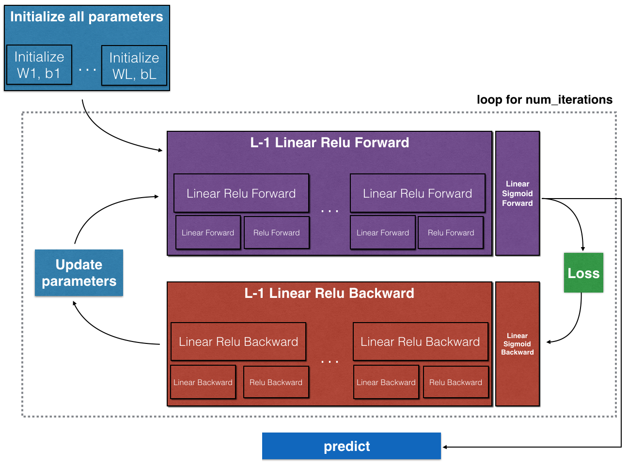
• Implement the forward propagation module (shown in purple in the figure below)
  • Complete the LINEAR part of a layer’s forward propagation step (resulting in $Z^{[l]}$)
  • Use ReLU/Sigmoid as the activation functions.
  • Combine the previous two steps into a new [LINEAR->ACTIVATION] forward function.
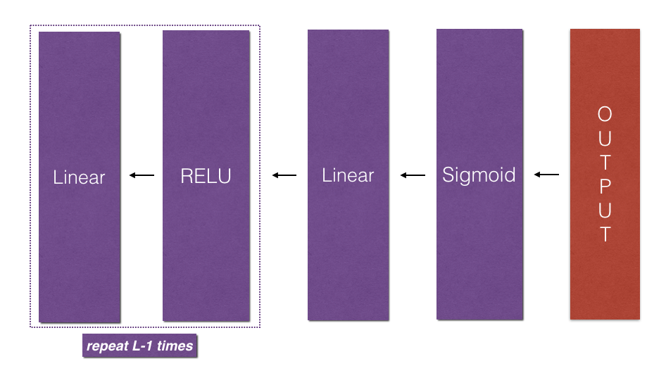
  • Stack the [LINEAR->RELU] forward function L-1 time (for layers 1 through L-1) and add a [LINEAR->SIGMOID] at the end (for the final layer $L$). This gives you a new L_model_forward function.
• Compute the loss
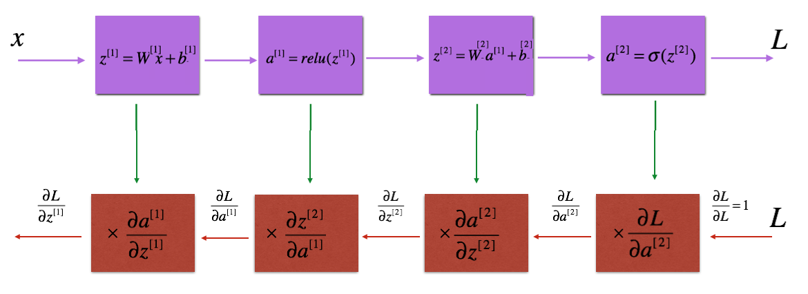
• Implement the backward propagation module (denoted in red in the figure below)
  • Complete the LINEAR part of a layer’s backward propagation step
  • USe relu_backward/sigmoid_backward to compute gradient of the activation functions
  • Combine the previous two steps into a new [LINEAR->ACTIVATION] backward function
  • Stack [LINEAR->RELU] backward L-1 times and add [LINEAR->SIGMOID] backward in a new L_model_backward function
• Update the parameters using gradient descent

Initialisation

Create and initialise the parameters of the 2-layer neural network with structure LINEAR -> RELU -> LINEAR -> SIGMOID.

def initialize_parameters(n_x, n_h, n_y):
    
    # Argument:
    # n_x -- size of the input layer
    # n_h -- size of the hidden layer
    # n_y -- size of the output layer
    
    # Returns:
    # parameters -- python dictionary containing your parameters:
    #                 W1 -- weight matrix of shape (n_h, n_x)
    #                 b1 -- bias vector of shape (n_h, 1)
    #                 W2 -- weight matrix of shape (n_y, n_h)
    #                 b2 -- bias vector of shape (n_y, 1)
    
    
    W1 = np.random.randn(n_h, n_x) * 0.01
    b1 = np.zeros((n_h, 1))
    W2 = np.random.randn(n_y, n_h) * 0.01
    b2 = np.zeros((n_y, 1))
    
    parameters = {"W1": W1,
                  "b1": b1,
                  "W2": W2,
                  "b2": b2}
    
    return parameters    

Let’s then initialise the parameters of an $L$-layer neural network with structure [LINEAR -> RELU] $\times$ (L-1) -> LINEAR -> SIGMOID.

def initialize_parameters_deep(layer_dims):
    
    # Arguments:
    # layer_dims -- python array (list) containing the dimensions of each layer in our network
    
    # Returns:
    # parameters -- python dictionary containing your parameters "W1", "b1", ..., "WL", "bL":
    #                 Wl -- weight matrix of shape (layer_dims[l], layer_dims[l-1])
    #                 bl -- bias vector of shape (layer_dims[l], 1)
    
    
    parameters = {}
    L = len(layer_dims) # number of layers in the network including the input layer

    for l in range(1, L):
        parameters['W' + str(l)] = np.random.randn(layer_dims[l], layer_dims[l-1]) * 0.01
        parameters['b' + str(l)] = np.zeros((layer_dims[l], 1))        
    return parameters

Forward Propagation

To do implement the forward propagation module properly, let’s write $3$ functions respectively to do the following:

• LINEAR
• LINEAR -> ACTIVATION where ACTIVATION will be either ReLU or Sigmoid.
• [LINEAR -> RELU] $\times$ (L-1) -> LINEAR -> SIGMOID (whole model)

Linear Forward

The linear forward module (vectorized over all the examples) computes the following equations:

\[Z^{[l]} = W^{[l]}A^{[l-1]} +b^{[l]}\]

where $A^{[0]} = X$.

def linear_forward(A, W, b):
    
    # Implement the linear part of a layer's forward propagation.
    # Arguments:
    # A -- activations from previous layer (or input data): (size of previous layer, number of examples)
    # W -- weights matrix: numpy array of shape (size of current layer, size of previous layer)
    # b -- bias vector, numpy array of shape (size of the current layer, 1)
    # Returns:
    # Z -- the input of the activation function, also called pre-activation parameter 
    # cache -- a python tuple containing "A", "W" and "b" ; stored for computing the backward pass efficiently
     
    Z = W @ A + b
    cache = (A, W, b)
    return Z, cache

Linear Activation Forward

In this project, we only use 2 activation functions:

• Sigmoid: $\sigma(Z) = \sigma(W A + b) = \frac{1}{ 1 + e^{-(W A + b)}}$.

  A, activation_cache = sigmoid(Z)
  

• ReLU: The mathematical formula for ReLu is $A = RELU(Z) = max(0, Z)$.

  A, activation_cache = relu(Z)
  

Now we implement the forward propagation of the LINEAR->ACTIVATION layer. Mathematically, $A^{[l]} = g(Z^{[l]}) = g(W^{[l]}A^{[l-1]} +b^{[l]})$ where the activation “g” can be sigmoid() or relu().

def linear_activation_forward(A_prev, W, b, activation):
   
    # Implement the forward propagation for the LINEAR->ACTIVATION layer
    # Arguments:
    # A_prev -- activations from previous layer (or input data): (size of previous layer, number of examples)
    # W -- weights matrix: numpy array of shape (size of current layer, size of previous layer)
    # b -- bias vector, numpy array of shape (size of the current layer, 1)
    # activation -- the activation to be used in this layer, stored as a text string: "sigmoid" or "relu"
    # Returns:
    # A -- the output of the activation function, also called the post-activation value 
    # cache -- a python tuple containing "linear_cache" and "activation_cache";
    #          stored for computing the backward pass efficiently
   
    
    if activation == "sigmoid":
        Z, linear_cache = linear_forward(A_prev, W, b)
        A, activation_cache = sigmoid(Z)
    
    elif activation == "relu":
        Z, linear_cache = linear_forward(A_prev, W, b)
        A, activation_cache = relu(Z)
    cache = (linear_cache, activation_cache)

    return A, cache

L Model Forward

It is time to put the above 2 functions together to implement the entire forward module. Mathematically, the variable AL will denote $A^{[L]} = \sigma(Z^{[L]}) = \sigma(W^{[L]} A^{[L-1]} + b^{[L]})$, where $\sigma$ stands for the sigmoid function.

def L_model_forward(X, parameters):
   
    # Implement forward propagation for the [LINEAR->RELU]*(L-1)->LINEAR->SIGMOID computation
    # Arguments:
    # X -- data, numpy array of shape (input size, number of examples)
    # parameters -- output of initialize_parameters_deep()
    # Returns:
    # AL -- activation value from the output (last) layer
    # caches -- list of caches containing:
    #             every cache of linear_activation_forward() (there are L of them, indexed from 0 to L-1)
   

    caches = []
    A = X
    L = len(parameters) // 2                  # number of layers in the neural network
    
    # Implement [LINEAR -> RELU]*(L-1). Add "cache" to the "caches" list.
    # The for loop starts at 1 because layer 0 is the input
    for l in range(1, L):
        A_prev = A 
        A, cache = linear_activation_forward(A_prev, parameters["W" + str(l)], parameters["b" + str(l)], 'relu')
        caches.append(cache)
    
    # Implement LINEAR -> SIGMOID. Add "cache" to the "caches" list.
    AL, cache = linear_activation_forward(A, parameters["W" + str(L)], parameters["b" + str(L)],'sigmoid')
    caches.append(cache)
          
    return AL, caches

Cost Function

We’ve implemented a full forward propagation that takes the input X and outputs a row vector $A^{[L]}$ containing the predictions. It also records all intermediate values in “caches”. Now we use $A^{[L]}$ to compute the cost of the predictions. This is straightforward as long as we are familiar with the formula of the logistic cost function.

The cost function is computed as

\[-\frac{1}{m} \sum\limits_{i = 1}^{m} \left[y^{(i)}\log\left(a^{[L] (i)}\right) + (1-y^{(i)})\log\left(1- a^{[L](i)}\right)\right].\]

def compute_cost(AL, Y):
    
    # Implement the cost function defined by equation (7).
    # Arguments:
    # AL -- probability vector corresponding to your label predictions, shape (1, number of examples)
    # Y -- true "label" vector (for example: containing 0 if non-cat, 1 if cat), shape (1, number of examples)
    # Returns:
    # cost -- cross-entropy cost
    
    
    m = Y.shape[1]
    cost = -1/m * np.sum(Y*np.log(AL) + (1-Y)*np.log(1-AL))
    cost = np.squeeze(cost)      # To make sure cost's shape is what we expect (e.g. this turns [[1]] into 1).

    return cost

Backward Propagation

Now, similarly to forward propagation, we build the backward propagation in three steps:

1. LINEAR backward
2. LINEAR -> ACTIVATION backward where ACTIVATION computes the derivative of either the ReLU or sigmoid activation
3. [LINEAR -> RELU] $\times$ (L-1) -> LINEAR -> SIGMOID backward (whole model)

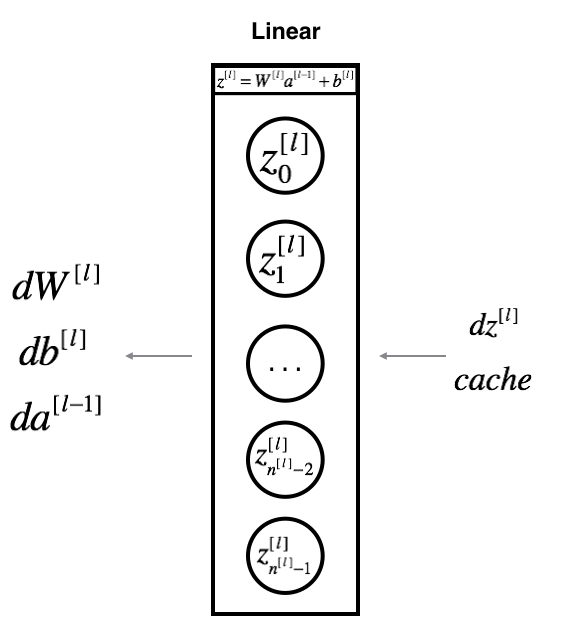
Linear Backward

Suppose we have already calculated the derivative $dZ^{[l]} = \frac{\partial \mathcal{L} }{\partial Z^{[l]}}$. We want to get $(dW^{[l]}, db^{[l]}, dA^{[l-1]})$. The three outputs $(dW^{[l]}, db^{[l]}, dA^{[l-1]})$ are computed using the input $dZ^{[l]}$.

Here are the formulas: \(dW^{[l]} = \frac{\partial \mathcal{J} }{\partial W^{[l]}} = \frac{1}{m} dZ^{[l]} A^{[l-1] T} \tag{8}\) \(db^{[l]} = \frac{\partial \mathcal{J} }{\partial b^{[l]}} = \frac{1}{m} \sum_{i = 1}^{m} dZ^{[l](i)}\tag{9}\) \(dA^{[l-1]} = \frac{\partial \mathcal{L} }{\partial A^{[l-1]}} = W^{[l] T} dZ^{[l]} \tag{10}\)

$A^{[l-1] T}$ is the transpose of $A^{[l-1]}$.

Note:

• axis=1 or axis=0 specify if the sum is carried out by rows or by columns respectively.
• keepdims specifies if the original dimensions of the matrix must be kept.

def linear_backward(dZ, cache):
    
    # Implement the linear portion of backward propagation for a single layer (layer l)

    # Arguments:
    # dZ -- Gradient of the cost with respect to the linear output (of current layer l)
    # cache -- tuple of values (A_prev, W, b) coming from the forward propagation in the current layer

    # Returns:
    # dA_prev -- Gradient of the cost with respect to the activation (of the previous layer l-1), same shape as A_prev
    # dW -- Gradient of the cost with respect to W (current layer l), same shape as W
    # db -- Gradient of the cost with respect to b (current layer l), same shape as b
    
    A_prev, W, b = cache
    m = A_prev.shape[1]

    dW = 1/m * dZ @ A_prev.T
    db = 1/m * np.sum(dZ, axis = 1, keepdims = True)
    dA_prev = W.T @ dZ
    
    return dA_prev, dW, db

Linear Activation Backward

Implement the backpropagation for the LINEAR->ACTIVATION layer. We already have the following 2 functions:

• sigmoid_backward: Implements the backward propagation for SIGMOID unit.

dZ = sigmoid_backward(dA, activation_cache)

• relu_backward: Implements the backward propagation for RELU unit.

dZ = relu_backward(dA, activation_cache)

If $g(.)$ is the activation function, sigmoid_backward and relu_backward compute

\[dZ^{[l]} = dA^{[l]} * g'(Z^{[l]}).\]

def linear_activation_backward(dA, cache, activation):
    
    # Implement the backward propagation for the LINEAR->ACTIVATION layer.
    
    # Arguments:
    # dA -- post-activation gradient for current layer l 
    # cache -- tuple of values (linear_cache, activation_cache) we store for computing backward propagation efficiently
    # activation -- the activation to be used in this layer, stored as a text string: "sigmoid" or "relu"
    
    # Returns:
    # dA_prev -- Gradient of the cost with respect to the activation (of the previous layer l-1), same shape as A_prev
    # dW -- Gradient of the cost with respect to W (current layer l), same shape as W
    # db -- Gradient of the cost with respect to b (current layer l), same shape as b
    
    linear_cache, activation_cache = cache
    
    if activation == "relu":
        dZ = relu_backward(dA, activation_cache)
        dA_prev, dW, db = linear_backward(dZ, linear_cache)
        
    elif activation == "sigmoid":
        dZ = sigmoid_backward(dA, activation_cache)
        dA_prev, dW, db = linear_backward(dZ, linear_cache)
    
    return dA_prev, dW, db

L Model Backward

Now we implement backpropagation for the [LINEAR->RELU] $\times$ (L-1) -> LINEAR -> SIGMOID model.

Recall that when we implemented the L_model_forward function, at each iteration, we stored a cache which contains (X,W,b, and z). In the back propagation module, we use those variables to compute the gradients. Therefore, in the L_model_backward function, we iterate through all the hidden layers backward, starting from layer $L$. On each step, we use the cached values for layer $l$ to backpropagate through layer $l$. The figure below shows the backward pass.

def L_model_backward(AL, Y, caches):
    
    # Implement the backward propagation for the [LINEAR->RELU] * (L-1) -> LINEAR -> SIGMOID group
    
    # Arguments:
    # AL -- probability vector, output of the forward propagation (L_model_forward())
    # Y -- true "label" vector (containing 0 if non-cat, 1 if cat)
    # caches -- list of caches containing:
    #             every cache of linear_activation_forward() with "relu" (it's caches[l], for l in range(L-1) i.e l = 0...L-2)
    #             the cache of linear_activation_forward() with "sigmoid" (it's caches[L-1])
    
    # Returns:
    # grads -- A dictionary with the gradients
    #          grads["dA" + str(l)] = ... 
    #          grads["dW" + str(l)] = ...
    #          grads["db" + str(l)] = ... 
    
    grads = {}
    L = len(caches) # the number of layers
    m = AL.shape[1]
    Y = Y.reshape(AL.shape) # after this line, Y is the same shape as AL
    dAL = - (np.divide(Y, AL) - np.divide(1 - Y, 1 - AL)) # derivative of cost with respect to AL    
    
    # Lth layer (SIGMOID -> LINEAR) gradients. Inputs: "dAL, current_cache". Outputs: "grads["dAL-1"], grads["dWL"], grads["dbL"]
    current_cache = caches[L - 1]
    dA_prev_temp, dW_temp, db_temp = linear_activation_backward(dAL, current_cache, 'sigmoid')
    grads["dA" + str(L-1)] = dA_prev_temp
    grads["dW" + str(L)] = dW_temp
    grads["db" + str(L)] = db_temp
    
    # Loop from l=L-2 to l=0
    for l in reversed(range(L-1)):
        # lth layer: (RELU -> LINEAR) gradients.
        # Inputs: "grads["dA" + str(l + 1)], current_cache". Outputs: "grads["dA" + str(l)] , grads["dW" + str(l + 1)] , grads["db" + str(l + 1)] 
        current_cache = caches[l]
        dA_prev_temp, dW_temp, db_temp = linear_activation_backward(grads["dA" + str(L-1)], current_cache, 'relu')
        grads["dA" + str(l)] = dA_prev_temp
        grads["dW" + str(l + 1)] = dW_temp
        grads["db" + str(l + 1)] = db_temp

    return grads

Update Parameters

To update the parameters of the model, we use the basic version of gradient descent:

\[W^{[l]} = W^{[l]} - \alpha \text{ } dW^{[l]},\] \[b^{[l]} = b^{[l]} - \alpha \text{ } db^{[l]},\]

where $\alpha$ is the learning rate.

After computing the updated parameters, we store them in the parameters dictionary.

def update_parameters(params, grads, learning_rate):
    
    # Update parameters using gradient descent
    
    # Arguments:
    # params -- python dictionary containing your parameters 
    # grads -- python dictionary containing your gradients, output of L_model_backward
    
    # Returns:
    # parameters -- python dictionary containing your updated parameters 
    #               parameters["W" + str(l)] = ... 
    #               parameters["b" + str(l)] = ...
    
    parameters = params.copy()
    L = len(parameters) // 2 # number of layers in the neural network

    # Update rule for each parameter. Use a for loop.
    for l in range(L):
        parameters["W" + str(l + 1)] = parameters["W" + str(l + 1)] - learning_rate * grads["dW" + str(l + 1)]
        parameters["b" + str(l + 1)] = parameters["b" + str(l + 1)] - learning_rate * grads["db" + str(l + 1)]

    return parameters

We are done! (In fact, not quite done yet. I will modify it later when I feel productive…) You can see an application of classifying cat vs non-cat images in this github repo.