The Derivative of Logistic Cost
Introduction
In machine learning, cost functions play a crucial role in training and evaluating models. They quantify the discrepancy between the predicted values and the labels, guiding the model towards optimal parameters. In this post, we will derive the derivative of cost function for logistic regression.
We start by looking at the linear regression model. Linear regression is a widely-used technique for predicting continuous values. The cost function used in linear regression is called the Mean Squared Error (MSE),
\[\text{MSE} = \frac{1}{m} \sum_{i=1}^{m}(\hat{y} - y)^2.\]where $\hat{y}$ represents the predicted values, $y$ represents the true labels, and $m$ is the number of training examples. It is straightforward to prove that this is a convex cost function and we can use gradient descent to find its global minimum. However, for logistic regression, using MSE results in a non-convex cost function with other local minima.
To preserve the convex nature of the cost function, we instead use the following cost function:
\[J(\mathbf{w}, b) = \frac{1}{m} \sum^m_{i=1}[-y^{(i)} \log(f_{\mathbf{w}, b}(\mathbf{x}^{(i)})) - (1-y^{(i)}) \log(1 - f_{\mathbf{w}, b}(\mathbf{x}^{(i)}))],\]where $f_{\mathbf{w}, b}(\mathbf{x}^{(i)}) = \frac{1}{1 + e^ {-(\mathbf{w} \cdot \mathbf{x} + b)}}$ is the sigmoid function. To use gradient descent to optimise, we need to find the derivatives of the logistic cost which are required in the backward propagation.
The derivative of the logistic cost
Let $w_j$ denote the $j$th component of $\mathbf{w}$ and similarly for $\mathbf{x}$. Then the partial derivative of $f_{\mathbf{w}, b}$ with respect to $w_j$ can be computed as follows:
\[\begin{align*} \frac{\partial}{\partial w_j}f_{\mathbf{w}, b} &= \frac{\partial}{\partial w_j} \left(\frac{1}{1 + e^ {-(\mathbf{w} \cdot \mathbf{x} + b)}}\right)\\ &= \frac{x_j^{(i)}e^{-(\mathbf{w} \cdot \mathbf{x} + b)} }{(1 + e^ {-(\mathbf{w} \cdot \mathbf{x} + b)})^2}\\ & = \frac{x_j^{(i)} - x_j^{(i)} + x_j^{(i)}e^{-(\mathbf{w} \cdot \mathbf{x} + b)} }{(1 + e^ {-(\mathbf{w} \cdot \mathbf{x} + b)})^2}\\ & = \frac{x_j^{(i)}}{1 + e^ {-(\mathbf{w} \cdot \mathbf{x} + b)}} \left( 1- \frac{1}{1 + e^ {-(\mathbf{w} \cdot \mathbf{x} + b)}} \right)\\ & = x_j^{(i)} f_{\mathbf{w}, b}(\mathbf{x}^{(i)}) \left(1- f_{\mathbf{w}, b}(\mathbf{x}^{(i)})\right). \end{align*}\]Hence, we also have
\[\begin{align*} \frac{\partial}{\partial w_j}\left(1 - f_{\mathbf{w}, b}\right) &= x_j^{(i)} f_{\mathbf{w}, b}(\mathbf{x}^{(i)}) \left(f_{\mathbf{w}, b}(\mathbf{x}^{(i)} - 1)\right). \end{align*}\]Combining these pieces, the partial derivative of the cost function $J$ with respect to $w_j$ is computed as
\[\begin{align*} \frac{\partial J}{\partial w_j} &= -\frac{1}{m} \sum^m_{i=1} \left[ \frac{y^{(i)}}{f_{\mathbf{w}, b}(\mathbf{x}^{(i)}) } x_j^{(i)} f_{\mathbf{w}, b}(\mathbf{x}^{(i)}) \left(1- f_{\mathbf{w}, b}(\mathbf{x}^{(i)})\right) + \frac{1 - y^{(i)}}{1 - f_{\mathbf{w}, b}(\mathbf{x}^{(i)}) } x_j^{(i)} f_{\mathbf{w}, b}(\mathbf{x}^{(i)}) \left(f_{\mathbf{w}, b}(\mathbf{x}^{(i)} - 1)\right) \right]\\ & = \frac{1}{m} \sum^m_{i = 1} \left[ y^{(i)} \left(1- f_{\mathbf{w}, b}(\mathbf{x}^{(i)})\right) + (1 - y^{(i)}) \left(f_{\mathbf{w}, b}(\mathbf{x}^{(i)} - 1)\right) \right]x_j^{(i)}\\ & = \frac{1}{m} \sum^m_{i = 1} \left( f_{\mathbf{w}, b}(\mathbf{x}^{(i)} - y^{(i)}) \right) x_j^{(i)}. \end{align*}\]In a similar manner,
\[\frac{\partial J}{\partial b} = \frac{1}{m} \sum^m_{i = 1} \left( f_{\mathbf{w}, b}(\mathbf{x}^{(i)} - y^{(i)}) \right).\]Gradient descent for logistic regression
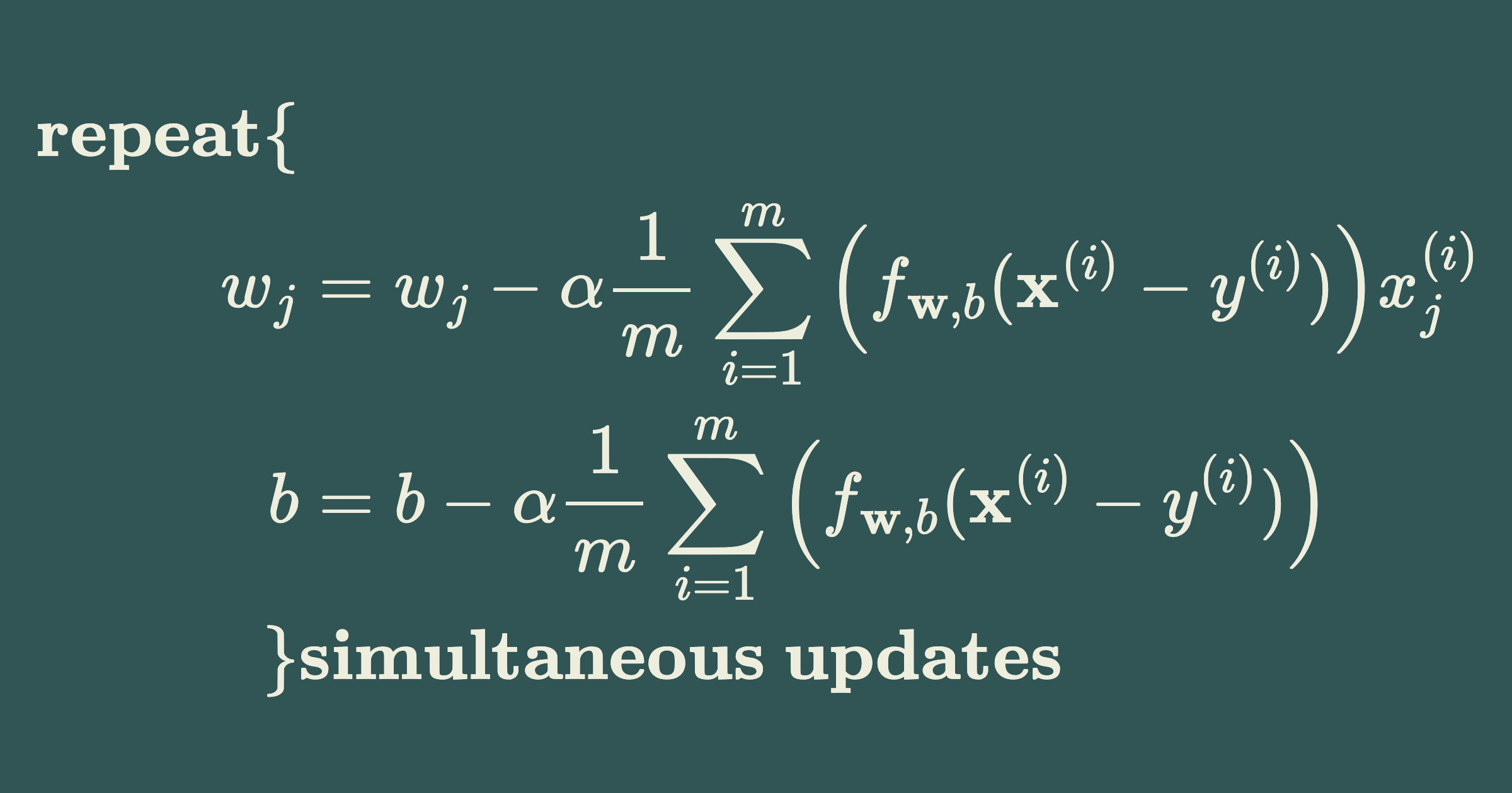
The gradient descent process can be performed as follows
\[\begin{align*} \textbf{repeat} \{\\ w_j &= w_j - \alpha \frac{1}{m} \sum^m_{i = 1} \left( f_{\mathbf{w}, b}(\mathbf{x}^{(i)} - y^{(i)}) \right) x_j^{(i)}\\ b &= b - \alpha \frac{1}{m} \sum^m_{i = 1} \left( f_{\mathbf{w}, b}(\mathbf{x}^{(i)} - y^{(i)}) \right)\\ \} &\textbf{simultaneous updates} \end{align*}\]