Splitting Graphs

Introduction
There are, in general, two ways to construct things in mathematics. On the one hand, we can construct things explicitly, which tends to be difficult, if we don’t know exactly what the target is. On the other hand, we can use an implicit construction, which is to say that we make some equation, show that it has a solution, and this solution is exactly what we want. However, there are certain problems we can’t solve using either of the above methods.
The “probabilistic method” for proving existence lies somewhere in the middle. We make a random object which with some probability $p$ being the object we want, and the existence of this object follows from by showing $p>0$.
Bipartite graphs and stable sets
Basic definitions
Definition 0.1 (Graph) A graph is a pair $G = (V, E)$ of sets, with $E \subseteq \binom{V}{2}$. We call elements of $V$ vertices and elements of $E$ edges.
We denote the vertices and edges of a graph $G$ by $V(G)$ and $E(G)$ repectively. The order of a graph is the number of its vertices $|V|$. The size of a graph is the number of edges $|E|$. Given a vertex $v \in V$, the neighbours of $v$ are $v’$ such that $\{v,v’\} \in E$. The degree, $deg(v)$, of vertex $v$ is the number of neighbours of $v$.
Lemma 0.2 For any graph $G = (V,E)$
\[\sum_{v\in V} d(v) = 2|E|.\]Proof: Summing the degree of all vertices is the same as counting each edge twice. ◼
Definition 0.3 (Bipartite graphs) A graph $G$ is bipartite if $V(G) = A \cup B$ where $A\cap B = \emptyset$ and $E(G) \subseteq \{ \{a,b\} | a \in A, b \in B\}$.
Definition 0.4 (Subgraphs) If $G$ and $H$ are graphs with $V(G) \subseteq V(G)$ and $E(H) \subseteq E(G)$, then $H$ is a subgraph of $G$.
An example of bipartite graphs
Example 0.5 Let $G = (V, E)$ be a graph with $m$ edges. Use the probabilitic method to show that $G$ has a bipartite subgraph containing at least $\frac{m}{2}$ edges.
 examples of bipartite graphs
Soln: Let $V_1 \subseteq V$ be a random subset where for each $x \in V$, we insert $x$ into $V_1$ with probability $p$, independently for each $x$. Let $V_2 = V \setminus V_1$. We call an edge $\{x, y\}$ crossing if one of $x, y$ are in $V_1$. Let $X$ be the number of crossing edges. Then
\[X = \sum_{\{x, y\} \in E} \mathbb{1}_{xy},\]where $\mathbb{1}_{xy}$ is the indicator random variable for $\{x,y\}$ being crossing. Then by the linearity of expectation,
\[\mathbb{E}[X] = \sum_{\{x, y\} \in E} \mathbb{E}[\mathbb{1}_{xy}] = 2mp(1-p).\]We now choose $p \in (0,1)$ to maximise this quantity. A bit of calculus finds that $p = \frac{1}{2}$ does the job, resulting in $\mathbb{E}[X] = \frac{m}{2}$. Thus, $\mathbb{P}[X = \frac{m}{2}] > 0$ and $X \geq \frac{m}{2}$ for some choice of $V_1$. ✓
Remark: One can choose a more subtle probability space to sharpen this bound.
An example of stable sets
Example 0.6 A stable set $S$ is a subset of $V$ such that no 2 elements of $S$ are neighbours. Let $d = \frac{2|E|}{|V|}$ and suppose that $d \geq 1$. Then show that $G$ contains a stable set of vertices with at least $\frac{|V|}{2d}$ elements.
 examples of stable sets in red
We first notice that $d$ is the average degree of vertices in $G$ (see lemma 0.2).
Soln: To make notation shorter, denote $|V| = n$ and $|E| = m$. Similar to the bipartite example, let $p \in (0,1)$ and $S$ be a random subset of $V$ where for each $v \in V$, $\mathbb{P}[v \in S] = p$, independently for each $v$. Notice that
\[|S| = \sum_{v \in V} \mathbb{1}_{\{v \in S\}},\]where $\mathbb{1}_{\{v \in S\}}$ is the indicator random variable for $v \in V$. Then by the linearity of expectation,
\(\mathbb{E}[|S|] = \sum_{v \in V} \mathbb{P}[v \in S] = np.\) The set $S$ we constructed has not to be a stable set. We want to know how close $S$ is to being a stable set. That is, we want to know how many vertices we need to remove from $S$ in order to make it into a stable set.
Let $Y = \{e \in E: \text{ both endpoints of }e \text{ are in } S \}$. If we take each edge $e \in Y$ and remove one of the endpoints of $e$ from $S$, then the result will be a stable set of size at least $|S| - |Y|$. The ‘at least’ comes from the possibility that the same vertex might be reckoned as an endpoint of more than one $e \in Y$. In symbols,
\[|Y| = \sum_{\{v, v'\} \in E} \mathbb{1}_{\{v\in S\}} \mathbb{1}_{\{v' \in S\}}\]So, by independence involved in the construction of $S$,
\[\mathbb{E}[|Y|] = \sum_{\{v, v'\} \in E} \mathbb{P}[v\in S, v' \in S] = \sum_{\{v, v'\} \in E} \mathbb{P}[v\in S] \mathbb{P}[v' \in S] = mp^2.\]Substituing $d = \frac{2m}{n}$, we have
\[\mathbb{E}[|S| - |Y|] = np(1-\frac{1}{2}dp).\]We now choose $p \in (0,1)$ to maximise this quantity. A bit of calculus finds that $p = \frac{1}{d}$ does the job, resulting in $E[|S| - |Y|] = \frac{n}{2d}$. Thus, $\mathbb{P}[|S| - |Y| = \frac{n}{2d}] > 0$. ✓
Exercise
Take a sphere of radius $1$, and a cube of radius $1$. $10\%$ of the surface of the sphere is coloured red and the rest is coloured black. Is it possible to inscribe the cube inside the sphere, such that all vertices of the cube are coloured black?

Hypergraph colouring
A colouring of a graph $G =(V, E)$ is an assignment of $k$ colours to $V$. The colouring is said to be proper if, for each edge $e$, the vertices at either end of $e$ are different colours. In this case, the colouring is generally referred to as a k-colouring of $G$. Let’s generalise this idea to hypergraphs.
Basic definitions
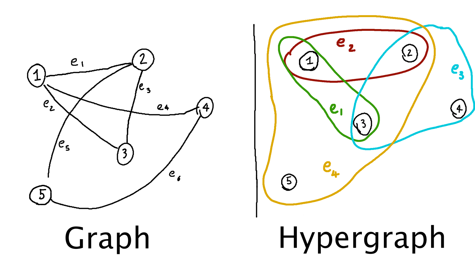
In a graph, each edge connects 2 vertices, so $e \in V \times V$. In a hypergraph a single edge connects multiple edges, so in this case we have $e \subseteq V$ and $E$ is a subset of the power set of $V$. We call elements of $E$, in this case, hyperedges.
 graph vs hypergraph
We update our definitions:
The degree, $deg(v)$, of the vertex $v \in V$ is the number of hyperedges which contain $v$. We say that a hypergraph is $k$-regular if each vertex has degree $k$.
The order of an edge, $|e|$, is the number of vertices contained inside this hyperedge. We say that a hypergraph is $k$-uniform if each edge has order $k$.
The colouring is proper, if for each edge e, the vertices inside $e$ are not all of the same colour. Note that $|e| = 2$ reduces to the definition for graphs.
For finite hypergraphs, $|V| < \infty$, it is clear that if $k = |V|$, then the hypergraph $G$ has a $k$-colouring, where we can simply take each vertex to be a different colour. A more interesting question is, can we find a $k$-colouring of $G$ with fewer colours?
We’ll show the following result in this post.
Lemma 0.7 Let $k \geq 9$ and let $G = (V, E)$ be a $k$-regular, $k$-uniform hypergraph. Then there exists a $2$-colouring of $G$.
To use probabilistic method as before, one can try colouring each vertex independently clour 1/colour 2 with some probability $p \in (0,1)$. Unfortunately, in this case the probability of getting a $2$-colouring is extremely small and we need a better idea, which comes from the following lemma.
Lemma 0.8 (Symmetric Lovász Local Lemma) Let $p \in (0,1)$ and $d \in \mathbb{N}$. Let $A_1,…, A_n$ be a sequence of events such that $\mathbb{P}[A_i] \leq p$ for all $i$, and each event is independent of all except $d$ of the others. If $\text{e}p(d + 1) \leq 1$, then $\mathbb{P}[A_1^c\cap A_2^c \cap … \cap A_n^c] > 0$.
Remark: The constant $\text{e}$ is the Euler’s constant which is approximately $2.72$. The power of Lemma 0.8 is that no matter how many events $(A_i)_{i=1}^n$ we have, it is possible to avoid all of them from happening. For those who are intersted, the proof of it will be in the next post as this post turned out to be a bit longer than I expected.
With Lemma 0.8 in hand, we can prove Lemma 0.7 quite easily.
Proof of Lemma 0.7: Independently colour each vertex $v \in V$ into colour 1 or colour 2 at random with probability $\frac{1}{2}$. For each hyperedge in $E$, let $A_e$ be the event that all vertices inside $e$ have the same colour. Since $G$ is $k$-uniform, we have $\mathbb{P}[A_e] = 2 \times \frac{1}{2^k} = 2^{1-k}$ for all $e \in E$.
Note that if $e, e’ \in E$ are two hyperedges with no vertices in common, then $A_e$ and $A_{e’}$ are independent. Any give hyperedge $e \in E$ contains $k$ vertices, and each such vertices can be contained in $k-1$ hyperedges excluding $e$ itself. Hence each event $A_e$ is independent of all other $A_{e’}$ except for $k(k-1)$ of them.
Applying Lemma 0.8 with $d = k(k-1)$ and $p = 2^{1-k}$, it remains to check if $\text{e}k(k-1)2^{1-k} \leq 1$ holds. The solutions to this inequality are $k \geq 8.40096$ or $x \in [-0.145232, 1.34737]$. Since we are given that $k \geq 9$, this inequality holds and implies that $\mathbb{P}[\cap_{e\in E}A^c_e] > 0$ and the $2$-colouring of $G$ exists.◼
You can show that Lemma 0.7 still hodls for $k \geq 4$ (Henning and Yeo [2013]), but the case $k = 2$ and $k = 3$ remain open.