Path Signatures
An introduction to path signatures, from rough path foundations to signature kernels and machine-learning applications.
Zhiyu Wang · Mathematical Institute, University of Oxford · March 2025
This article is the web-readable version of the presentation prepared for the Department of Mathematics. The complete slides are also available below.
Time-ordered data
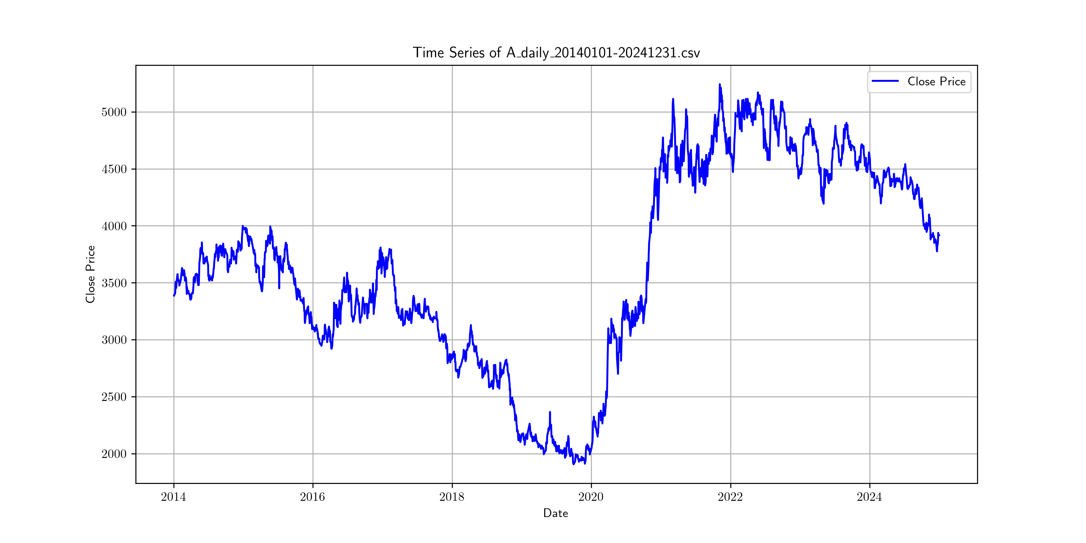
Financial times-series.
Text: “The quick brown fox jumped over the lazy dog.”
Time-evolving network.

Time-ordered data as paths
We can think of time-ordered data as a path, i.e. a continuous function
\[X:[a, b] \rightarrow E\]for some set \(E\) (target space).
Financial time series: \(X:[a, b] \rightarrow \mathbb{R}^d,[a, b]=\) time horizon, \(d=\) number of assets tracked;
Text: \(X:[0, T] \rightarrow \mathcal{A}, T=\) length of text, \(\mathcal{A}=\{a, A, b, B, \ldots\}=\) alphabet;
Time-evolving network: \(X:[0, T] \rightarrow \mathcal{G}, \mathcal{G}=\) a set of graphs.
Features of paths
We would like to summarise important features of paths.
Goal: introduce a special feature, the signature of a path, which have desired properties listed below.
Sometimes only the order \(X_{t_1}, \ldots, X_{t_N}\) matters and the time-paramterisation \(\left(t_1, \ldots, t_N\right)\) is irrelevant (Time-representation invariance);
One-to-one correspondence between paths and their features (Uniqueness);
We observe only finitely many points \(\left\{X_{t_i}\right\}_{i=1}^N\), not the whole path \(\left\{X_t\right\}_{t \in[0, T]}\) (Factorial decay).
Applications
The signature method has been
combined with convolutional neural nets (CNNs) to win first prize in ICDAR 2013 Online Isolated Chinese Character recognition competition;
combined with gradient boosting regression to win first prize in PhysioNet 2019 Computing in Cardiology Challenge;
combined with graph convolutional networks (GCNs) for Skeleton-Based Action Recognition;
combined with generative adversarial networks (GANs) under the conditional Sig-Wasserstein framework for time series generation…
Outline
Rough Path Theory and Signatures
Properties of Path Signatures
Paths
Paths form one of the basic elements of this chapter. Let us first introduce the concepts of continuous \(E\)-valued paths and finite \(p\)-variation paths. Let \((E, \| \cdot \|_E)\) be a finite dimensional real Banach space with \(\text{dim}(E) = d\).
Definition (Path). A path is a continuous function \(X : [a, b] \to E\).
We use the subscript notation \(X_t=X(t)\) to denote dependence on \(t \in[a, b]\) and superscript notation to denote its coordinates \(X_t = (X_t^1, X_t^2, \dots, X_t^d)\) We denote the space of all continuous paths by \(\mathsf{C}^0([a, b], E)\).
\(p\)-variation
Definition (\(p\)-variation of a path). Let \(p \geq 1\) be a real number. Let \(X: [a, b] \to E\) be a continuous path. The \(p\)-variation of \(X\) on the interval \([a, b]\) is defined by
\[\|X\|_{p, [a, b]}=\left[\sup _{a \leq t_0 \leq \ldots \leq t_r \leq b} \sum_{j=0}^{r-1}\left\|X_{t_j}-X_{t_{j+1}}\right\|^p_E\right]^{\frac{1}{p}}.\]
Remark. A Brownian motion \(B : [a, b] \to \mathbb{R}\) has finite \(p\)-variation for \(p>2\). Yet, the \(2\)-variation of \(B\) is almost surely infinite as proven in (Freedman 1971).
Topology on path space
Let \(\mathcal{V}^p\left([a, b], E\right)\) denote the space of continuous paths \(X: [a, b] \rightarrow E\) of finite \(p\)-variation, i.e.
\[\mathcal{V}^p\left([a, b], E\right) = \{X \in \mathsf{C}^0([a, b], E) \mid \|X\|_{p, [a, b]} < \infty\}.\]Paths of finite \(1\)-variation are also called bounded variation paths.
It is easy to check that the \(p\)-variation \(\|\cdot\|_{p,[a, b]}\) is a seminorm and not a norm as all constant paths have zero \(p\)-variation. To rectify this, we can define the \(p\)-variation norm on \(\mathcal{V}^p\left([a, b], E\right)\) by
\[\|X\|_{\mathcal{V}^p}=\|X\|_{p,[a, b]}+\sup _{t \in[a, b]}\left\|X_t\right\|.\]Proposition. \(\left(\mathcal{V}^p\left([a, b], E\right), \|\cdot\|_{\mathcal{V}^p}\right)\) is a Banach space.
Tensor algebra
It turns out that the path signature which we will define later possesses a rich algebraic structure encapsulated by the tensor algebra.
Definition (Extended tensor algebra/Space of formal series; (Lyons et al. 2007, Definition 2.4)). The extended tensor algebra of \(E\), denoted by \(T((E))\), is the direct (Cartesian) product
\[T((E)):= \prod_{i = 0}^{\infty} {E}^{\otimes i} = \left\{\boldsymbol{a}=\left(a_0, a_1, \ldots, a_n, \ldots\right) \mid a_n \in {E}^{\otimes n}\right\}.\]Here, \(E^{\otimes n}=\underbrace{E \otimes \cdots \otimes E}_{n \text { times }}\) denotes the \(n\)-fold tensor product of \(E\) with itself. By convention, \(E^{\otimes 0}:=\mathbb{R}\).
Extended tensor algebra as a vector space and beyond
\(T((E))\) is naturally equipped with a vector space structure. Let \(\boldsymbol{a}=\left(a_0, a_1, \ldots\right)\) and \(\boldsymbol{b}=\left(b_0, b_1, \ldots\right)\) be two elements of \(T((E))\). Let \(\lambda \in \mathbb{R}\). Define the addition and scalar multiplication as follows:
\[\boldsymbol{a}+\boldsymbol{b}=\left(a_0+b_0, a_1+b_1, \ldots\right) \quad \text{and} \quad \lambda \boldsymbol{a} = \left(\lambda a_0, \lambda a_1, \ldots\right).\]Moreover, this vector space becomes a real unital algebra if we define the product of \(\boldsymbol{a}\) and \(\boldsymbol{b}\) as
\[\boldsymbol{a} \otimes \boldsymbol{b}=\left(c_0, c_1, \ldots\right), \quad c_n=\sum_{k=0}^n a_k \otimes b_{n-k} \quad \forall \, n \in \mathbb{N}.\]In fact, we can define norms and inner products on \(T((E))\). We will discuss this later.
Subspaces of extended tensor algebra
Definition. Let \(T_{1}((E))\) be the subset of \(T((E))\) where
\[T_{1}((E)):=\left\{\left(a_0, a_1, a_2, \ldots\right) \in T((E)) \mid a_0=1\right\}.\]
Proposition. \((T_{1}((E)), \otimes)\) is a group.
Tensor algebra
Definition (Tensor algebra; (Lyons et al. 2007, Definition 2.5)). The tensor algebra over \(E\) is the direct sum of \(n\)-fold tensor products
\[T((E)) \supset T(E) := \bigoplus_{i=0}^{\infty} {E}^{\otimes i}= \left\{\boldsymbol{a}=\left(a_k\right)_{k=0}^{\infty} \mid a_k \in E^{\otimes k}, \exists N \in \mathbb{N} \text{ s.t. } a_k=0 \, \forall k \geq N\right\}.\]
Remark. Note that an element in \(T((E))\) is an infinite sequence of possibly infinitely many non-zero tensors, while an element in \(T(E)\) is an infinite sequence of finitely many non-zero tensors. In other words, \(T(E)\) is a proper subset of \(T((E))\).
Truncated tensor algebra
Definition (Truncated tensor algebra). The truncated tensor algebra at order \(n \in \mathbb{N}\) is
\[T(E) \supseteq T^{(n)}(E):=\bigoplus_{i=0}^{n} E^{\otimes i}= \left\{\boldsymbol{a}=\left(a_k\right)_{k=0}^{\infty} \mid a_k \in E^{\otimes k}, a_k=0 \, \forall k \geq n\right\}.\]
The product \(\otimes\) given by (tensor-product formula) is also defined on \(T^{(n)}(E)\) for \(0 \leq k \leq n\). Moreover, note that the dimension of the truncated tensor algebra at order \(n\) is given by
\[\operatorname{dim}\left(T^{(n)}(E)\right)=\sum_{i=0}^n d^i=\frac{d^{n+1}-1}{d-1}.\]Intuitive understanding of \(E^{\otimes n}\)
Remark. Informally, we view the \(0\)-fold tensor product \(E^{\otimes 0}\) as the set of all scalars \(a_0 \in \mathbb{R}\) with dimension \(d^0 = 1\). Similarly, \(E^{\otimes 1}\) is the set of real vectors \(v \in E\) with dimension \(d^1 = d\) and \(E^{\otimes 2}\) is the set of real matrices \(A \in \mathbb{R}^{d \times d}\) with dimension \(d^2\). Thus, a zero tensor at level \(2\) can be understood as the zero matrix and more formally, let \(\{e_{i_1} \otimes e_{i_2} \otimes \cdots \otimes e_{i_n} \mid 0 \leq i_1 \leq m_1, \dots, 0 \leq i_n \leq m_n\}\) be a basis of \(E^{\otimes n}\), then the zero tensor is
\[0=\sum_{0 \leq i_1 \leq m_1, \dots, 0 \leq i_n \leq m_n} 0 \cdot\left(e_{i_1} \otimes e_{i_2} \otimes \cdots \otimes e_{i_n}\right).\]
Canonical homomorphism
Definition (Canonical homomorphism). Let \(n \in \mathbb{N}\). The canonical homomorphism is
\[\pi_n: T((E)) \rightarrow T^{(n)}(E), \quad\left(a_0, a_1, \ldots\right) \mapsto\left(a_0, a_1, \ldots, a_n, 0, \dots \right).\]
Word
Before formally defining path signatures, let us first introduce the concepts of word and Young integral.
Definition (Words). A word is a finite tuple
\[\mathcal{W}(\mathcal{A}_d) \ni \mathsf{I}=\left(i_1, \ldots, i_k\right)=: i_1 \ldots i_k\]with \(i_1, \ldots, i_k \in\{1, 2, \ldots, d\}\). The length of word \(\mathsf{I}\) is \(\lvert\mathsf{I}\rvert:=k\). The set \(\mathcal{A}_d := \{1, 2, \ldots, d\}\) is the alphabet. Moreover, denote by \(\mathcal{W}(\mathcal{A}_d)\) the countably infinite set of all words on the alphabet \(\mathcal{A}_d\)
\[\mathcal{W}\left(\mathcal{A}_d\right):=\{\emptyset, 1, \ldots, d, 11, \ldots, dd, \ldots\}.\]
An example of words
Example (\(d = 3\)). Let \(\mathcal{A}_3 = \{1,2,3\}\) be the alphabet. Then
\[\mathcal{W}(\mathcal{A}_3) = \{\emptyset,1,2,3,11,12,13,21,22,23,31,32,33,111,112,113,121, \ldots\}.\]
Young integrals
Since the paths in our discussion are all \(E\)-valued, we need a suitable framework for integration along paths in Banach spaces. This is provided by the Young integral. Given Banach spaces \(V\) and \(W\), the Young integral determines a way for a path \([a, b] \rightarrow \mathcal{L}(V, W)\) to be integrated along a path \([a, b] \rightarrow V\). The notation \(\mathcal{L}(V, W)\) denotes the space of bounded linear operators \(V \rightarrow W\). To be more precise, let \(X:[a, b] \rightarrow V\) and \(Y:[a, b] \rightarrow \mathcal{L}(V, W)\). Given a partition \(\mathcal{D}=\left(a=t_0, t_1, \ldots, t_r=b\right)\) of \([a, b]\) we let \(\lvert\mathcal{D}\rvert:=\min \left\{t_{i+1}-t_i \mid i \in\{0, \ldots, r-1\}\right\}\). We first define
\[\int_{\mathcal{D}} Y d X:=\sum_{i=0}^{r-1} Y_{t_r}\left(X_{t_{r+1}}-X_{t_r}\right)\]Then, given \(t \in[a, b]\), the Young integral of \(Y\) along \(X\) over the interval \([a, t]\) is defined as
Young integrals (continued)
\[\int_a^t Y_s d X_s:=\lim _{j \rightarrow \infty} \int_{\mathcal{D}_j} Y d X\]where \(\left\{\mathcal{D}_j\right\}_{j=1}^{\infty}\) is a sequence of partitions of \([a, t]\) with \(\left\lvert\mathcal{D}_j\right\rvert \rightarrow 0\) as \(j \rightarrow \infty\). Formally, we have the following theorem.
Theorem (Young; (Lyons et al. 2007, Theorem 1.16)). Let \(V\) and \(W\) be two Banach spaces. Let \(p, q \in \mathbb{R}_{\geq 1}\) with \(\frac{1}{p}+\frac{1}{q}>1\), \(X \in \mathcal{V}^p([a, b], V)\), and \(Y \in \mathcal{V}^q([a, b], \mathcal{L}(V, W))\). Then, for each \(t \in[a, b]\), the limit
\[\int_0^t Y_s d X_s=\lim _{\lvert\mathcal{D}\rvert \rightarrow 0, \, \mathcal{D} \subset[a, t]} \int_{\mathcal{D}} Y d X\]exists. Moreover, the mapping \(t \mapsto \int_a^t Y_s d X_s\) belongs to \(\mathcal{V}^p([a, b], W)\).
Coordinate iterated integrals
Definition (Iterated integral). For \(p \in [1, 2)\), \(X \in \mathcal{V}^p\left([a, b], E\right)\), word \(\mathsf{I}=i_1 \ldots i_k\), and domain \([s,t] \subseteq [a, b]\), the iterated integral \(S(X)_{s, \boldsymbol{\cdot}}^\mathsf{I}\) is defined inductively by
\[\mathcal{V}^p([a, b], E) \ni S(X)_{s, \boldsymbol{\cdot}}^{\mathsf{I}}=\int_s^{\boldsymbol{\cdot}} S(X)_{s, u}^{i_1 \ldots i_{k-1}} dX_u^{i_k}, \quad S(X)_{s, t}^{\emptyset}=1.\]
An example of iterated integrals
Example. We can explicitly write out the iterated integral as follows:
\[\begin{aligned} & S(X)_{s, t}^{\emptyset}=1, \quad S(X)_{s, t}^i=\int_s^t dX_u^i=X_t^i-X_s^i, \\ & S(X)_{s, t}^{ij}=\int_s^t \int_s^u d X_v^i d X_u^j, \quad S(X)_{s, t}^{i j k}=\int_s^t \int_s^{t_3} \int_s^{t_2} d X_{t_1}^i d X_{t_2}^j d X_{t_3}^k. \end{aligned}\]Generally, one has
\[S(X)_{s, t}^{i_1 \ldots i_k}=\int_s^t \int_s^{t_k} \cdots \int_s^{t_2} dX_{t_1}^{i_1} \ldots dX_{t_{k-1}}^{i_{k-1}} d X_{t_k}^{i_k}.\]
Signature coefficients
To make our notation compact, we use the signature coefficient.
Definition (Signature coefficient). With the notation as above, define the signature coefficient \(S(X)_{s, t}^{i_1 \ldots i_k}\) indexed by word \(i_1 \ldots i_k \in \mathcal{W}(\mathcal{A}_d)\) as
\[E \ni S(X)_{s, t}^{i_1 \ldots i_k}:= \int_{s<t_1<\cdots<t_k<t} d X_{t_1}^{i_1} \cdots d X_{t_k}^{i_k}= \int_s^t \int_s^{t_k} \cdots \int_s^{t_2} dX_{t_1}^{i_1} d X_{t_1}^{i_1} \ldots d X_{t_k}^{i_k}.\]
Signature of finite \(p\)-variation paths with \(p \in [1,2)\)
Now we are ready to give the definition of the signature of finite \(p\)-variation paths with \(p \in [1,2)\). The path signature is indexed by words.
Definition (Signature I). Let \(p \in [1,2)\) and \(X \in \mathcal{V}^p\left([a, b], E\right)\). The signature \(S(X)_{s, t}\) of \(X\) over domain \([s, t] \subseteq[a, b]\) is the infinite set of real numbers indexed by words \(\mathsf{I} \in \mathcal{W}(\mathcal{A}_d)\)
\[\left\{ S(X)_{s, t}^\mathsf{I}\right\}_{I \in \mathcal{W}} =\{\underbrace{S_{s, t}^{\emptyset}}_1, \underbrace{S(X)_{s,t}^1}_{X_b^1-X_a^1}, \ldots, \underbrace{S(X)_{s,t}^d}_{X_b^d-X_a^d}, S(X)_{s,t}^{11}, S(X)_{s,t}^{12},\ldots, S(X)_{s,t}^{d d}, S(X)_{s,t}^{111}, \ldots \}.\]
Signature of finite \(p\)-variation paths with \(p \in [1,2)\)
Observe that there is a natural grading on the signature \(S(X)_{s,t}\) based on the length of indexed words. With a slight abuse of notation, we have
\[S(X)_{s, t}=\left\{1 , S_{s, t}^{[1]}(X), S_{s, t}^{[2]}(X), \ldots\right\}, \quad S(X)_{s, t}^{[k]}=\left\{S(X)_{s, t}^\mathsf{I}\right\}_{\lvert\mathsf{I}\rvert=k}.\]Thus, the signature can be elegantly encoded as an element in the extended tensor algebra \(T((E))\). We present the following alternative definition of the signature.
Signature of finite \(p\)-variation paths with \(p \in [1,2)\)
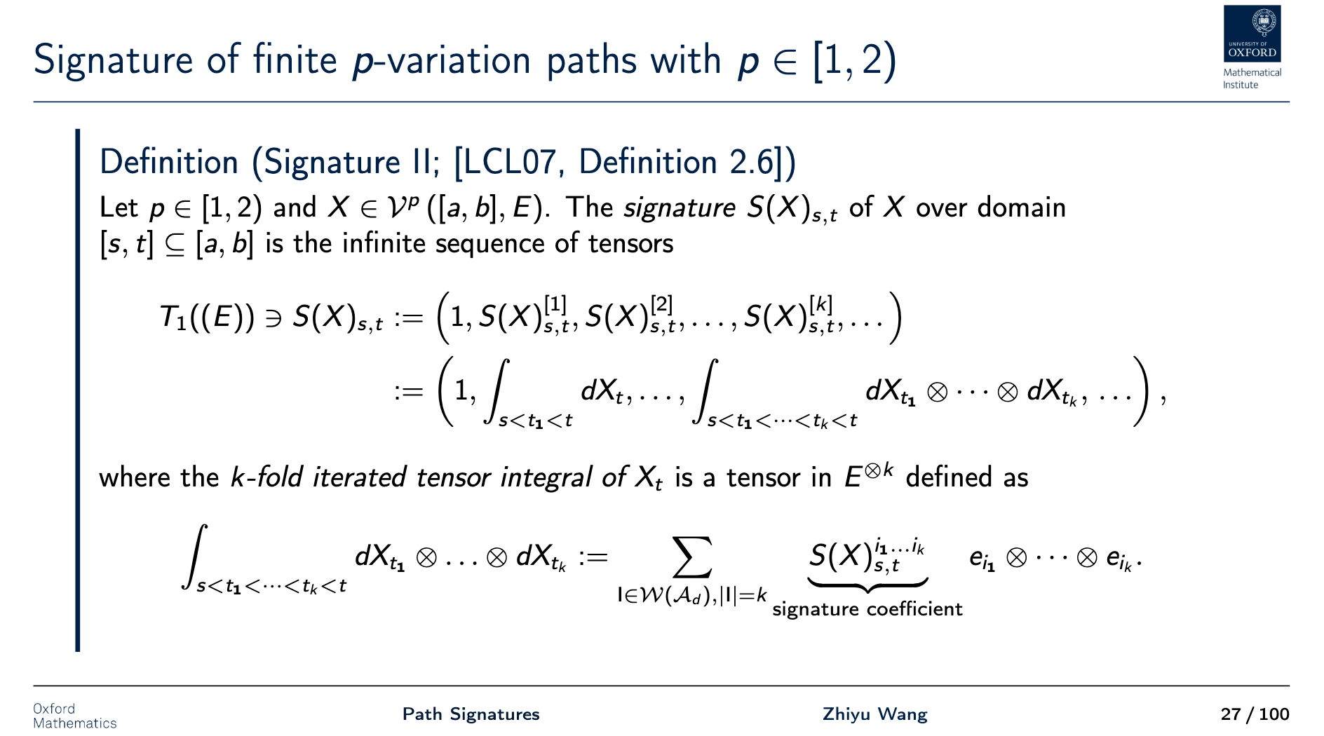
Definition (Signature II; (Lyons et al. 2007, Definition 2.6)). Let \(p \in [1,2)\) and \(X \in \mathcal{V}^p\left([a, b], E\right)\). The signature \(S(X)_{s, t}\) of \(X\) over domain \([s, t] \subseteq [a, b]\) is the infinite sequence of tensors
\[\begin{aligned} T_{1}((E)) \ni S(X)_{s, t} & := \left(1, S(X)_{s, t}^{[1]}, S(X)_{s, t}^{[2]}, \dots, S(X)_{s, t}^{[k]}, \dots \right)\\ &:= \left(1, \int_{s<t_1<t} d X_t, \ldots, \int_{s<t_1<\cdots<t_k<t} d X_{t_1} \otimes \cdots \otimes d X_{t_k}, \, \ldots\right), \end{aligned}\]where the \(k\)-fold iterated tensor integral of \(X_t\) is a tensor in \({E}^{\otimes k}\) defined as
\[\int_{s<t_1<\cdots<t_k<t} d X_{t_1} \otimes \ldots \otimes d X_{t_k} := \sum_{\mathsf{I} \in \mathcal{W}(\mathcal{A}_d), \lvert\mathsf{I}\rvert=k} \underbrace{S(X)_{s, t}^{i_1 \ldots i_k}}_{\text{signature coefficient}} e_{i_1} \otimes \cdots \otimes e_{i_k}.\]
Examples of path signatures
Example (Linear path). Let \(x \in E\) and define \(X_t=t x\) for \(t \in[0,1]\). We have
\[S(X)_{0,1}^{i_1 \ldots i_k}=\frac{x^{i_1} \ldots x^{i_k}}{k!} .\]
Example (One-dimensional path). Consider \(X \in \mathcal{V}^1([a, b], E)\). We have
\[S(X)_{a, b}^{1 \ldots 1}=\frac{\left(X_b-X_a\right)^k}{k!} .\]Hence \(S(X)_{a, b}\) only captures the increment for one-dimensional paths.
Truncated signatures
Definition (Truncated signature). Let \(n \in \mathbb{N}_{+}\). The level-\(n\) truncated signature is defined as
\[T^{(n)}(E) \ni S^{(n)}(X)_{s, t}=\pi_n\left(S(X)_{s, t}\right).\]
Remark. Note that \(S^{[n]}(X)_{s, t} \in E^{\otimes n}\) while \(S^{(n)}(X)_{s, t} \in\) \(T^{(n)}(E)\).
Geometric properties
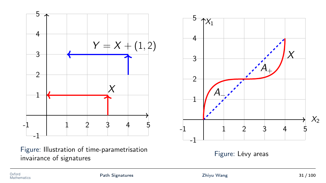
Proposition (Time-parametrisation invariance). Consider \(X \in \mathcal{V}^{1}\left([a, b], E\right)\) and a non-decreasing bijection \(\psi:[x, y] \rightarrow[a, b]\). Define \(Y \in \mathcal{V}^1\left([x, y], E\right)\) by \(Y_t=X_{\psi(t)}\). Then
\[S(X)_{a, b}=S(Y)_{x, y}.\]
Proposition (Base-point invariance). Consider \(X \in \mathcal{V}^1\left([a, b], E\right)\) and \(h \in E\). Define \(Y \in \mathcal{V}^1\left([a, b], E\right)\) as \(Y_t=X_t+h\). Then
\[S(X)_{a, b}=S(Y)_{a, b}.\]
Geometric illustrations
Geometric properties (continued)
Definition (Lévy area). The Lévy area of a \(2\)-dimensional path \(X = (X^1, X^2) \in \mathcal{V}^1\left([a, b], \mathbb{R}^2\right)\) is the real number \(A_{+} - A_{-}\).
Proposition (2nd order signatures compute Lévy area). One has
\[S(X)_{a, b}^{12}-S(X)_{a, b}^{21}=2\left(A_{+}-A_{-}\right).\]
Algebraic properties
Proposition (Chen’s identity). Let \(X \in \mathcal{V}^{1}\left([a, b], E\right)\) and \(c \in [a, b]\). One has
\[S(X)_{a, b} = S(X)_{a, c} \otimes S(X)_{c, b}.\]
Remark. If we were to use Definition (Signature I) to formalise Chen’s identity, then we would have had a much more cumbersome form
\[S(X)_{a, b}^{i_1 \ldots i_k}=\sum_{m=0}^k S(X)_{a, c}^{i_1 \ldots i_m} S(X)_{c, b}^{i_{m+1} \ldots i_k}, \quad \forall \, i_1 \ldots i_k \in \mathcal{W}(\mathcal{A}_d).\]
Concatenation of paths
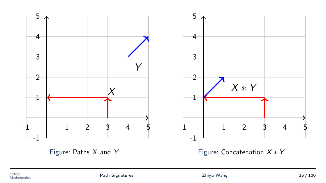
Definition (Concatenation of paths). For \(X, Y \in \mathcal{V}^1\left([0,1], E\right)\), define their concatenation \(X * Y \in \mathcal{V}^1\left([0,1], E\right)\)
\[(X * Y)_t:= \begin{cases}X_{2 t} & \text { if } t \in[0,1 / 2], \\ X_1+\left(Y_{2 t-1}-Y_0\right) & \text { if } t \in[1 / 2,1].\end{cases}\]
Proposition (Chen’s identity for concatenation of paths). We have \(S(X)_{0,1} \otimes S(Y)_{0,1}=S(X * Y)_{0,1}\).
Concatenation of paths
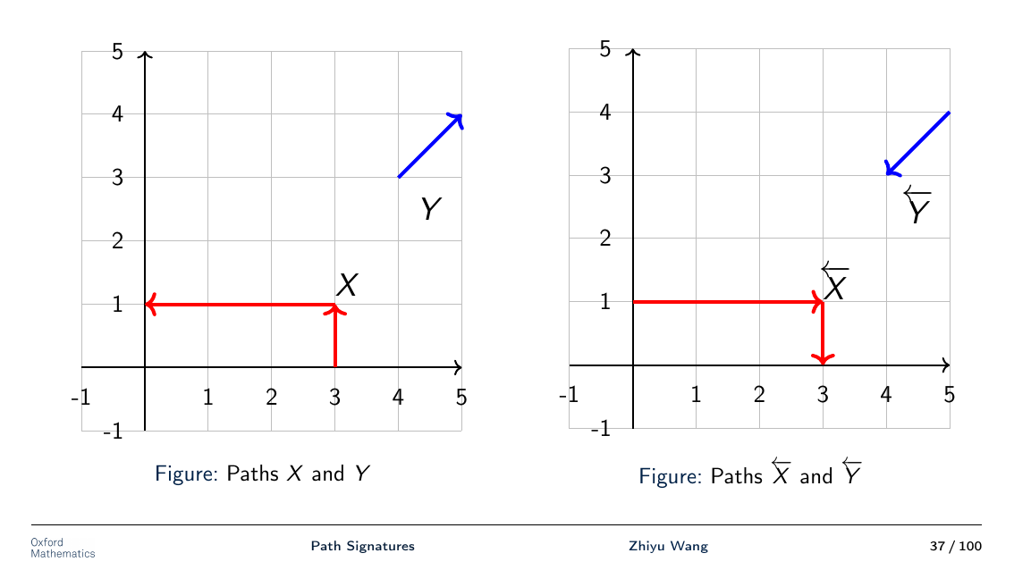
Time reversal of a path
Definition (Time reversal). For a path \(X:[a, b] \to E\) in \(\mathcal{V}^1\left([0,1], E\right)\), define its time-reversal \(\overleftarrow{X}:[a, b] \to E\) by \(\overleftarrow{X}_t=X_{a+b-t}\) for all \(t \in[a, b]\).
Proposition. We have
\[S(X)_{a, b} \otimes S(\overleftarrow{X})_{a, b}= \mathbf{1}.\]Equivalently,
\[S(X)_{a, b}^{i_1 \ldots i_k}=(-1)^k S(\overleftarrow{X})_{a, b}^{i_k \ldots i_1}.\]
Time reversal illustrations
A detour to shuffle products
Definition (\((k,m)\)-shuffle). For \(k, m \in \mathbb{N}\), a permutation \(\sigma\) of \(\{1, \ldots, k+m\}\) is a \((k, m)\)-shuffle if
\[\sigma^{-1}(1)<\ldots<\sigma^{-1}(k) \quad \text {and} \quad \sigma^{-1}(k+1)<\ldots<\sigma^{-1}(k+m).\]Let \(\operatorname{Shuffles}(k, m) \subseteq \mathcal{S}_{k+m}\) denote the set of all \((k, m)\)-shuffles.
Definition (Shuffle product). Consider two words \(\mathsf{I, J} \in \mathcal{W}(\mathcal{A}_d)\) where \(\mathsf{I}=i_1 \ldots i_k\) and \(\mathsf{J}=j_1 \ldots j_m\). Let word \(\mathsf{R}\) be given by
\[\mathsf{R} = r_1 \ldots r_k r_{k+1} \ldots r_{k+m}=i_1 \ldots i_k j_1 \ldots j_m.\]The shuffle product of \(\mathsf{I}\) and \(\mathsf{J}\) is the finite multiset of words
\[\mathsf{I} \mathbin{\sqcup\!\sqcup} \mathsf{J}=\left\{\!\!\!\left\{r_{\sigma(1)} \ldots r_{\sigma(k+m)} \mid \sigma \in \operatorname{Shuffles}(k, m)\right\}\!\!\!\right\}.\]
Algebraic properties (continued)
Example. \(\textcolor{red}{121} \mathbin{\sqcup\!\sqcup} \textcolor{blue}{23}=\{\!\!\{ \textcolor{red}{121}\textcolor{blue}{23},\textcolor{red}{12}\textcolor{blue}{2}\textcolor{red}{1}\textcolor{blue}{3},\textcolor{red}{1}\textcolor{blue}{2}\textcolor{red}{21}\textcolor{blue}{3},\textcolor{blue}{2}\textcolor{red}{121}\textcolor{blue}{3},\textcolor{red}{12}\textcolor{blue}{23}\textcolor{red}{1},\textcolor{red}{1}\textcolor{blue}{2}\textcolor{red}{2}\textcolor{blue}{3}\textcolor{red}{1},\textcolor{blue}{2}\textcolor{red}{12}\textcolor{blue}{3}\textcolor{red}{1},\textcolor{red}{1}\textcolor{blue}{23}\textcolor{red}{21}, \textcolor{blue}{2}\textcolor{red}{1}\textcolor{blue}{3}\textcolor{red}{21},\textcolor{blue}{23}\textcolor{red}{121}\}\!\!\}\)
Proposition (Shuffle product identity). For \(X \in \mathcal{V}^1\left([a, b], E\right)\) and words \(\mathsf{I, J} \in \mathcal{W}(\mathcal{A}_d)\), one has
\[S(X)_{a, b}^\mathsf{I} S(X)_{a, b}^\mathsf{J}=\sum_{\mathsf{K} \in \mathsf{I} \mathbin{\sqcup\!\sqcup} \mathsf{J}} S(X)_{a, b}^\mathsf{K}.\]
Example. For \(X \in \mathcal{V}^1\left([a, b], E\right)\), we have
\[S(X)_{a, b}^{\textcolor{red}{12}} S(X)_{a, b}^{\textcolor{blue}{23}}= S(X)_{a, b}^{\textcolor{red}{12}\textcolor{blue}{23}}+S(X)_{a, b}^{\textcolor{red}{1}\textcolor{blue}{2}\textcolor{red}{2}\textcolor{blue}{3}}+S(X)_{a, b}^{\textcolor{blue}{2}\textcolor{red}{12}\textcolor{blue}{3}} +S(X)_{a, b}^{\textcolor{red}{1}\textcolor{blue}{23}\textcolor{red}{2}}+S(X)_{a, b}^{\textcolor{blue}{2}\textcolor{red}{1}\textcolor{blue}{3}\textcolor{red}{2}}+S(X)_{a, b}^{\textcolor{blue}{23}\textcolor{red}{12}}.\]
Extended tensor algebra as a normed space
Recall that \((E, \| \cdot \|_E)\) is a Banach space. In order to equip the extended tensor algebra \(T((E))\) with a norm, we define admissible tensor norms.
Definition (Admissible tensor norm; (Lyons et al. 2007, Definition 1.25)). A family of norms on \(E^{\otimes n}\) with \(n \in \mathbb{N}_{+}\) is admissible if
For \(n \in \mathbb{N}_{+}\), the norm \(\|\cdot\|_{E^{\otimes n}}\) on \(E^{\otimes n}\) is invariant under the action of the symmetric group \(S_n\) on \(E^{\otimes n}\), i.e.
\[\forall n \in \mathbb{N}_{+} \, \forall x \in E^{\otimes n} \, \forall \rho \in S_n, \|\rho(x)\|_{E^{\otimes n}}=\|x\|_{E^{\otimes n}}.\]Here, for \(\rho \in S_n\) and \(a_1 \otimes \ldots \otimes a_n \in E^{\otimes n}\), then \(\rho\left(a_1 \otimes \ldots \otimes a_n\right):=a_{\rho(1)} \otimes \ldots \otimes a_{\rho(n)}\) and is extended to the entirety of \(E^{\otimes n}\) by linearity.
For \(n, m \in \mathbb{N}_{+}\), the norm \(\|\cdot\|_{E^{\otimes n}}\) is submultiplicative, i.e.
\[\forall n, m \in \mathbb{N}_{+} \, x, y \in E^{\otimes n}, \|x \otimes y\|_{E^{\otimes(n+m)}} \leq\|x\|_{E^{\otimes n}}\|y\|_{E^{\otimes m}}.\]
Extended tensor algebra as a normed space (continued)
Now we can define a norm on \(T((E))\) by
\[\|v\|_{T((E))}:=\sum_{n=0}^{\infty}\left\|\pi_n(v)\right\|_{E^{\otimes n}}.\]With the properties of the admissible tensor norm \(\|\cdot\|_{E^{\otimes n}}\), one can check that \(\|\cdot\|_{T((E))}\) is indeed a norm on \(T((E))\).
Controls
Let \(\Delta_{[a, b]}:=\{(s, t) \in \mathbb{R}^2 \mid a \leq s \leq t \leq b\}\) be a simplex.
Definition (Control; (Lyons et al. 2007, Definition 1.9)). A control on \([a,b]\) is a continuous function \(\omega : \Delta_{[a, b]} \to [0, \infty)\) such that
\(\omega\) is super-additive, i.e.
\[\forall s, t, u \in [a, b] \text{ with } s \leq u \leq t, \omega(s, u)+\omega(u, t) \leq \omega(s, t);\]\(\omega\) vanishes on the diagonal, i.e.
\[\forall t \in [a, b], \omega(t, t) = 0.\]
Examples of controls
Example. Let \(p \in \mathbb{R}_{\geq 1}\) and \(X \in \mathcal{V}^p([a, b], E)\). Define \(\omega_X: \Delta_{[a, b]} \rightarrow [0, \infty)\) as
\[\omega_X(s, t):=\|X\|_{p,[s, t]}^p = \sup _{\mathcal{D} \subset[s, t]} \sum_{i=0}^{r-1}\left\|X_{t_i}-X_{t_{i+1}}\right\|_E^p.\]Then \(\omega_X\) is a control.
Upper estimates
Proposition. Let \(p \in[1,2)\) and \(X \in \mathcal{V}^p([a, b], E)\). Then there exists a control \(\omega: \Delta_{[a, b]} \rightarrow [0, \infty)\) such that for every \(n \in \mathbb{N}_{+}\) and every \((s, t) \in \Delta_{[a, b]}\), we have
\[\left\|S^{[n]}(X)_{s, t}\right\|_{E^{\otimes n}} \leq \frac{\omega(s, t)^n}{\Gamma\left(1+\frac{n}{p}\right)},\]where \(\Gamma(\cdot)\) is the Gamma function.
Factorial decay
Corollary (Factorial decay; (Lyons et al. 2007, Proposition 2.2)). For \(p = 1\), we have for every \(n \in \mathbb{N}_{+}\) and every \((s, t) \in \Delta_{[a, b]}\)
\[\left\|S^{[n]}(X)_{s, t}\right\|_{E^{\otimes n}} \leq \frac{\|X\|_{1,[s, t]}^n}{n!}.\]
Consequently, truncating the signature to a finite depth effectively captures the most significant terms in a norm-based sense. We will see later that this factorial decay property not only reduces computational complexity but also makes it feasible to use signatures as features in machine learning models.
Height functions
Definition (Height function; (Hambly and Lyons 2010, Definition 1.3)). Given a path \(X:[a, b] \rightarrow\) \(E\), a height function for \(X\) is a non-negative continuous function \(h:[a, b] \rightarrow \mathbb{R}\) such that \(h(a)=h(b)=0\) and
\[\left\|X_t-X_s\right\| \leq h(s)+h(t)-2 \inf _{u \in[s, t]} h(u) \text { for all } a \leq s<t \leq b.\]
Tree-like equivalence
Definition (Tree-like path; (Hambly and Lyons 2010, Definition 1.3)). A bounded variation path is called tree-like if it has a height function.
Definition (Tree-like equivalence; (Hambly and Lyons 2010, Definition 1.4)). Let \(X, Y \in \mathcal{V}^1([a, b], E)\). \(X\) and \(Y\) are tree-like equivalent if \(X * \overleftarrow{Y}\), the concatenation of \(X\) with the reversed path of \(Y\), is a tree-like path. We denote it by \(X \sim Y\).
Proposition. Tree-like equivalence \(\sim\) is an equivalence relation.
Tree-like paths
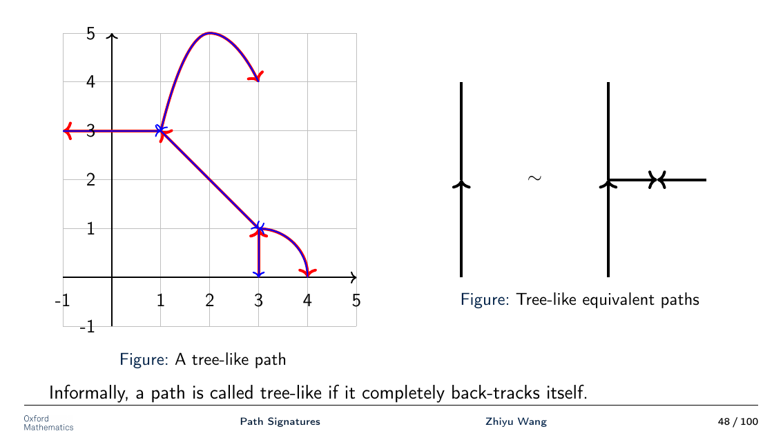
Informally, a path is called tree-like if it completely back-tracks itself.
Signature determines paths up to tree-like equivalence
Theorem (Uniqueness of the signature). Let \(X, Y \in \mathcal{V}^1([a, b], E)\). Then \(X\) is tree-like equivalent to \(Y\) if and only if \(S(X)=S(Y)\).
The following proposition is a useful sufficient condition for the uniqueness of the signature.
Proposition. Let \(X \in \mathcal{V}^1([a, b], E)\) with a fixed starting point and at least one coordinate of \(X\) is a monotone function. Then \(S(X)\) determines \(X\) uniquely.
Quotient space of bounded variation paths \(\mathcal{P}^1([a,b], E)\)
One of the most fundamental results in the study of the signature is its universal nonlinearity, which states that continuous functions on path space can be well approximated by linear functionals on the signature. We first define a quotient space of bounded variation paths modulo the tree-like equivalence relation.
Definition. Define \(\mathcal{P}^1([a,b], E) := \mathcal{V}^1([a, b], E)/\sim\). Any element in \(\mathcal{P}^1([a,b], E)\) is an equivalence class \([X]\) for some \(X \in \mathcal{V}^1([a, b], E)\). By Theorem uniqueness theorem, we define the signature of \([X] \in \mathcal{P}^1([a,b], E)\) as the signature of any representative \(\tilde{X} \in \mathcal{V}^1([a, b], E)\) of the equivalence class \([X]\).
Topology on \(\mathcal{P}^1([a,b], E)\)
Definition ((Lyons and Qian 2002) (Equation (3.70))). Given \([X], [Y] \in \mathcal{P}^1([a,b], E)\), define
\[d_{\mathcal{P}^1}([X],[Y]):= \sup _{a \leq t_0 \leq \ldots \leq t_r \leq b}\left(\sum_{j=0}^{r-1}\left\|S(X)^1_{t_j, t_{j+1}}-S(Y)^1_{t_j, t_{j+1}}\right\|_{E }\right),\]where \(S(X)^1_{t_j, t_{j+1}}\) and \(S(Y)^1_{t_j, t_{j+1}}\) are signature coefficients defined as in Definition signature-coefficient definition.
Remark. Theorem (Uniqueness of the signature) ensures that (path-space metric) is well-defined.
Signature is a universal approximator of continuous functions
Theorem (Universal Nonlinearity). Let \(\mathcal{K} \subset \mathcal{P}^1([a, b], E)\) be compact and \(f: \mathcal{K} \rightarrow \mathbb{R}\) a continuous function with respect to the topology generated by (path-space metric). Then for any \(\varepsilon>0\) there exists a truncation level \(k \in \mathbb{N}\) and \(\alpha_{i, \mathsf{I}} \in \mathbb{R}\) such that for all \(X \in \mathcal{K}\)
\[\left\lvert f(x)-\sum_{i=0}^k \sum_{\mathsf{I} \in \mathcal{W}(\mathcal{A}_d)} \alpha_{i, \mathsf{I}} S(X)_{a, b}^\mathsf{I}\right\rvert \leq \varepsilon.\]
Neural networks are universal approximators
Theorem ((Paluzo-Hidalgo et al. 2020, Theorem 1)). \(\sigma\) is not polynomial iff for every continuous function \(f: K \subset \mathbb{R}^d \rightarrow \mathbb{R}\) defined on a compact set \(K\) and \(\varepsilon>0\), there exists a two-layer neural network with \(m\) neurons and weights \(\mathbf{W}, \mathbf{b}, \mathbf{v}\) s.t.
\[\max _{x \in K}\left\lvert f(x)-\sum_{j \leq m} v_j \sigma\left(w_j^{\mathrm{T}} x+b_j\right)\right\rvert<\varepsilon\]
Fixed number of layers (“bounded depth”)
Does not tell how many neurons \(m\) are needed (“arbitrary width”)
There are stronger results, including bounded depth and width
Exponential function on extended tensor algebra
Definition (Tensor exponential). The tensor exponential \(\exp: T((E)) \to T((E))\) is defined as
\[T((E)) \ni \exp (\boldsymbol{a}):=\sum_{n=0}^{\infty} \frac{\boldsymbol{a}^{\otimes n}}{n!} = \boldsymbol{1}+\boldsymbol{a}+\frac{\boldsymbol{a}^{\otimes 2}}{2!}+\frac{\boldsymbol{a}^{\otimes 3}}{3!}+\cdots,\]where \(\boldsymbol{1} = (1, 0, 0, \dots)\).
Remark. The exponential series defined above is convergent as shown in (Lyons et al. 2007, Lemma 2.19) in the sense that the level-\(k\) tensor of \(\exp (\boldsymbol{a})\) converges in \(E^{\otimes k}\) under the admissible tensor norm \(\|\cdot\|_{E^{\otimes k}}\).
Logarithm function on extended tensor algebra
Definition (Tensor logarithm). The tensor logarithm \(\log: T_{>0}((E)) \to T((E))\) is defined as
\[T((E)) \ni \log (\boldsymbol{a}):=\log \left(\pi_0(\boldsymbol{a})\right)+\sum_{n=1}^{\infty} \frac{(-1)^n}{n}\left(\boldsymbol{1}-\frac{\boldsymbol{a}}{\pi_0(\boldsymbol{a})}\right)^{\otimes n},\]where \(\boldsymbol{1} = (1, 0, 0, \dots)\) and \(\pi_0 : T((E)) \to \mathbb{R}\) is the canonical homomorphism.
Remark. On the other hand, the tensor logarithm series is well-defined above as it only contains finitely many terms at each level. This can be seen by noting that
\[\boldsymbol{1}-\frac{\boldsymbol{a}}{\pi_0(\boldsymbol{a})} = \left(0, -\frac{\pi_1(\boldsymbol{a})}{\pi_0(\boldsymbol{a})} \dots \right)\]and hence \(\left(\boldsymbol{1}-\frac{\boldsymbol{a}}{\pi_0(\boldsymbol{a})}\right)^{\otimes n}_k = 0\) for all \(k < n\).
Exp and Log are inverses of each other
Moreover, if we restrict the tensor exponential and logarithm on certain subsets, then they are inverses of each other.
Recall that \(T_{1}((E)):=\left\{\left(a_0, a_1, a_2, \ldots\right) \in T((E)) \mid a_0 = 1\right\}\). Similarly, let \(T_{>0}((E)):=\left\{\left(a_0, a_1, a_2, \ldots\right) \in T((E)) \mid a_0>0\right\}\) and \(T_{0}((E)):=\left\{\left(a_0, a_1, a_2, \ldots\right) \in T((E)) \mid a_0=0\right\}\).
Proposition. The restricted exponential and logarithm function \(\exp: T_0((E)) \to T_1((E))\) and \(\log: T_{1}((E)) \to T_0((E))\) are bijective and inverses of each other.
Signatures have redundancy
Shuffle product identity \(\Rightarrow\) signature terms not algebraically independent. Recall the example we have seen earlier:
Example. For \(X \in \mathcal{V}^1\left([a, b], E\right)\), we have
\[S(X)_{a, b}^{\textcolor{red}{12}} S(X)_{a, b}^{\textcolor{blue}{23}}= S(X)_{a, b}^{\textcolor{red}{12}\textcolor{blue}{23}}+S(X)_{a, b}^{\textcolor{red}{1}\textcolor{blue}{2}\textcolor{red}{2}\textcolor{blue}{3}}+S(X)_{a, b}^{\textcolor{blue}{2}\textcolor{red}{12}\textcolor{blue}{3}} +S(X)_{a, b}^{\textcolor{red}{1}\textcolor{blue}{23}\textcolor{red}{2}}+S(X)_{a, b}^{\textcolor{blue}{2}\textcolor{red}{1}\textcolor{blue}{3}\textcolor{red}{2}}+S(X)_{a, b}^{\textcolor{blue}{23}\textcolor{red}{12}}.\]
To remove this redundancy, we introduce the Log signature.
Log signatures and truncated log signature
Definition (Log signature). Let \(p \in [1,2)\) and \(X \in \mathcal{V}^p\left([a, b], E\right)\). The log signature \(\mathrm{log}S(X)_{s, t}\) of \(X\) over domain \([s, t] \subseteq [a, b]\) is
\[T_0((E)) \ni \mathrm{log} S(X)_{s, t} := \sum_{n=1}^{\infty} \frac{(-1)^n}{n}\left(\boldsymbol{1}-S(X)_{s, t}\right)^{\otimes n}.\]
Definition (Truncated log signature). Let \(n \in \mathbb{N}_{+}\). The level-\(n\) truncated log signature is defined as
\[T^{(n)}(E) \ni \mathrm{log}^{(n)}S(X)_{s, t}=\pi_n\left(\mathrm{log}S(X)_{s, t}\right).\]
Lie algebra
Definition (Lie algebra). A Lie algebra \(\mathfrak{g}\) over \(\mathbb{R}\) is a real vector space with a map \([\cdot, \cdot]: \mathfrak{g} \times \mathfrak{g} \rightarrow \mathfrak{g}\) called the Lie bracket such that
the Lie bracket \([\cdot, \cdot]\) is bilinear;
\([x, y]=-[y, x]\);
Jacobi’s identity holds: \([x,[y, z]]+[y,[z, x]]+[z,[x, y]]=0\).
Proposition. Let \([\cdot, \cdot]:T((E)) \times T((E)) \to T((E))\) be defined as
\[[\boldsymbol{a}, \boldsymbol{b}] = \boldsymbol{a} \otimes \boldsymbol{b}-\boldsymbol{b} \otimes \boldsymbol{a}.\]Then \(\left( T((E)), [\cdot, \cdot] \right)\) forms a Lie algebra.
Subspaces generated by lie brackets
Definition. Let \(F_1\) and \(F_2\) be subspaces of \(T((E))\). Define
\[\left[F_1, F_2\right]:=\operatorname{span}\left(\left\{[\boldsymbol{a}, \boldsymbol{b}] \mid \boldsymbol{a} \in F_1 \text{ and } \boldsymbol{b} \in F_2\right\}\right).\]
Now a sequence of subspaces \((L_i)_{i=0}^{\infty}\) of \(T((E))\) can be recursively defined as
\[L_0=\{0\}, \quad L_1=E, \quad L_2=\left[E, L_1\right]=[E, E], \quad L_3=\left[E, L_2\right]=[E,[E, E]], \quad \ldots,\]and generally, \(L_{n+1}:=\left[E, L_n\right] \subset E^{\otimes(n+1)}\).
Log signatures live in the space of lie formal series
Definition (Lie formal series; (Lyons et al. 2007, Definition 2.22)). The space of Lie formal series over \(E\) is the subspace \(\mathcal{L}((E)) \subset T((E))\) given by
\[\mathcal{L}((E)):=\left\{\boldsymbol{l} \in T((E)) \mid \forall n \in \mathbb{Z}_{\geq 0}, \, \pi_n(\boldsymbol{l}) \in L_n\right\}.\]Moreover, for \(n \in \mathbb{N}\) we define the Lie polynomials of degree \(n\) to be the subset
\[\mathcal{L}^{(n)}(E):= \pi_n(\mathcal{L}((E))) = \bigoplus_{i=0}^{n} L_i.\]
Proposition. We have \(\mathrm{log} S(X)_{s, t} \in \mathcal{L}((E))\) and \(\mathrm{log}^{(n)}S(X)_{s, t} \in \mathcal{L}^{(n)}(E)\).
Rough paths
Note that we have only defined the signature of finite \(p\)-variation paths with \(p \in [1,2)\). In the case where \(p \geq 2\), we need a new framework beyond the Young integral.
For instance, for a Brownian motion, on the other hand, the integrals can be understood in the sense of Itô or Stratonovich.
- \[G \Omega_p(E) \subset W G \Omega_p(E) \subset \Omega_p(E)\]
- We can define the signature of a p-rough paths
Kernel Learning
Evaluation functionals
Definition (Evaluation functional). Let \(\mathcal{H} \subseteq \mathbb{R}^{\mathcal{X}}\) be a Hilbert space of functions. The evaluation functional at a fixed \(x \in \mathcal{X}\) is the map
\[\delta_x: \mathcal{H} \rightarrow \mathbb{R}, \quad f \mapsto f(x).\]
Remark. Evaluation functionals are always linear. For \(f, g \in \mathcal{H}\) and \(\lambda \in \mathbb{R},\) we have \(\delta_x(f+\lambda g)=( f+ \lambda g)(x)= f(x)+ \lambda g(x)= \delta_x(f)+ \lambda \delta_x(g)\). However, evaluation functionals are not always continuous.
An example of discontinuous evaluation functional
Example (Discontinuous evaluation functional). Let \(\mu\) be the Lebesgue measure on \(\mathbb{R}\). Consider the Hilbert space \((L^2([0,1];\mu), \|\cdot\|_{L^2})\) of square integrable equivalence classes of functions where \(\forall f_1, f_2 \in L^2([0,1])\),
\[\left\|f_1-f_2\right\|_{L^2}=\left(\int_0^1\left\lvert f_1(x)-f_2(x)\right\rvert^2 d \mu(x)\right)^{\frac{1}{2}}.\]Now, observe that the sequence of monomials \(\left(q_n\right)_{n=1}^{\infty}\) with \(q_n=x^n\) converges to the zero function in \(L^2\) norm since
\[\lim _{n \rightarrow \infty}\left\|q_n-0\right\|_{L^2}= \lim _{n \rightarrow \infty}\left(\int_0^1 x^{2 n} d x\right)^{\frac{1}{2}} = \lim _{n \rightarrow \infty} \frac{1}{\sqrt{2 n+1}} =0\]but does not converge pointwise at \(x = 1\) since
\[1=\lim _{n \rightarrow \infty} \delta_1\left(q_n\right) \neq \delta_1\left(\lim _{n \rightarrow \infty} q_n\right)=0.\]
Reproducing kernel Hilbert spaces
Definition (RKHS). A Hilbert space of functions \(\mathcal{H} \subseteq \mathbb{R}^{\mathcal{X}}\) is a Reproducing Kernel Hilbert Space (RKHS) if the evaluation functional \(\delta_x\) is continuous for all \(x \in \mathcal{X}\).
Remark. It may seem evident from Example (Discontinuous evaluation functional) that \(L^2([0,1];\mu)\) is not an RKHS. However, it fails to be a valid counterexample since it consists of equivalence classes of functions rather than individual functions, and thus is not strictly a space of functions. Consequently, it does not even fall within the scope of the discussion. Only by invoking the Axiom of Choice can one provide a non-constructive proof of the existence of a Hilbert space of functions that is not an RKHS.
Functions are well-behaved in RKHSs
A notable consequence is that RKHSs exhibit particularly well-behaved properties compared to general Hilbert spaces of functions. Specifically, we have the property that two functions close in RKHS norm implies that they are also close posintwise.
Proposition ((Berlinet and Thomas-Agnan 2004, Corollary 1)). Let \(\mathcal{H} \subseteq \mathbb{R}^{\mathcal{X}}\) be an RKHS. If \(\lim _{n \rightarrow \infty}\left\|f_n-f\right\|_{\mathcal{H}}=0\), then \(\lim _{n \rightarrow \infty} f_n(x)= f(x)\) for all \(x \in \mathcal{X}\).
Reproducing kernels
The definition of an RKHS in does not explicitly mention a kernel. We now introduce reproducing kernels, kernels, and positive semi-definite functions to illustrate how they relate to RKHSs.
Definition (Reproducing kernel; (Berlinet and Thomas-Agnan 2004, Definition 1)). Let \(\mathcal{H} \subseteq \mathbb{R}^{\mathcal{X}}\) be a Hilbert space of functions. A bivariate function \(k: \mathcal{X} \times \mathcal{X} \rightarrow \mathbb{R}\) is a reproducing kernel of \(\mathcal{H}\) if
\(\forall x \in \mathcal{X}, k(\cdot, x) \in \mathcal{H}\);
reproducing property holds: \(\forall x \in \mathcal{X} \, \forall f \in \mathcal{H}, \langle f, k(\cdot, x)\rangle_{\mathcal{H}}=f(x).\)
Existence and uniqueness of reproducing kernels
Proposition (Existence of reproducing kernel; (Berlinet and Thomas-Agnan 2004, Theorem 1)). Let \(\mathcal{H} \subseteq \mathbb{R}^{\mathcal{X}}\) be a Hilbert space of functions. Then \(\mathcal{H}\) is an RKHS if and only if there exists a reproducing kernel of \(\mathcal{H}\).
Proposition (Uniqueness of reproducing kernel). Let \(\mathcal{H} \subseteq \mathbb{R}^{\mathcal{X}}\) be an RKHS. The reproducing kernel of \(\mathcal{H}\) is unique.
Positive semi-definite functions
Let us now characterise reproducing kernels with positive semi-definite functions.
Definition (Positive semi-definite function; (Berlinet and Thomas-Agnan 2004, Definition 2)). A bivariate function \(k: \mathcal{X} \times \mathcal{X} \rightarrow \mathbb{R}\) is positive semi-definite if \(k\) is symmetric and for any \((x_i)_i^{n} \subseteq \mathcal{X}, (\alpha_i)_{i=1}^n \subseteq \mathbb{R}\)
\[\sum_{i=1}^n \sum_{j=1}^n \alpha_i \alpha_j k\left(x_i, x_j\right) \geq 0.\]
Relation to positive semi-definite matrices
Remark. One can immediately see that a bivariate function \(k: \mathcal{X} \times \mathcal{X} \rightarrow \mathbb{R}\) is positive semi-definite if and only if the Gram matrix of \(k\)
\[K := \left[ \begin{array}{ccc} k(x_1, x_1) & \cdots & k(x_1, x_n) \\ \vdots & \ddots & \vdots \\ k(x_n, x_1) & \cdots & k(x_n, x_n) \end{array} \right]\]is positive semi-definite for any \((x_i)_i^{n} \subseteq \mathcal{X}\).
Inner products are positive semi-definite
In fact, every inner product is a positive semi-definite function. More generally, we have this following useful proposition.
Proposition. Let \(\mathcal{H}\) be a Hilbert space and \(\phi: \mathcal{X} \rightarrow \mathcal{H}\). Then the bivariate function \(h: \mathcal{X} \times \mathcal{X} \to \mathbb{R}\)
\[h(x, y) = \langle\phi(x), \phi(y)\rangle_{\mathcal{H}}\]is positive semi-definite.
Corollary ((Berlinet and Thomas-Agnan 2004, Lemma 2)). Let \(\mathcal{H} \subseteq \mathbb{R}^{\mathcal{X}}\) be an RKHS. The reproducing kernel \(k: \mathcal{X} \times \mathcal{X} \to \mathbb{R}\) of \(\mathcal{H}\) is a positive semi-definite function.
Kernels
Kernel methods are a versatile algorithmic framework which allows construction of nonlinear machine learning algorithms by employing linear tools in a nonlinearly transformed feature space. Let us now introduce the definition of a kernel.
Definition (Kernel; (Steinwart and Christmann 2008, Definition 4.1)). A bivariate function \(k: \mathcal{X} \times \mathcal{X} \rightarrow \mathbb{R}\) is a kernel if there exists a Hilbert space \(\mathcal{H}\) called feature space and a feature map \(\varphi: \mathcal{X} \rightarrow \mathcal{H}\) such that for any \(x, x^{\prime} \in \mathcal{X}\)
\[k\left(x, x^{\prime}\right)=\langle \varphi(x), \varphi\left(x^{\prime}\right) \rangle_{\mathcal{H}} .\]
Proposition. Kernels are positive semi-definite functions.
Proposition (Reproducing kerenls are kernels; (Steinwart and Christmann 2008, Lemma 4.19)). Let \(\mathcal{H} \subseteq \mathbb{R}^{\mathcal{X}}\) be an RKHS. The reproducing kernel of \(\mathcal{H}\) is a kernel.
Feature maps and linear separation
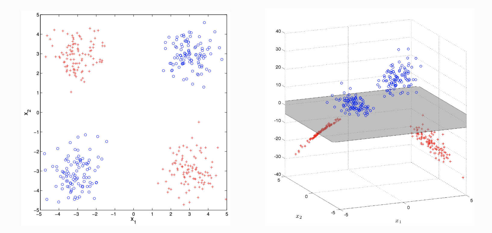
No linear classifier separates red from blue.
Linear separation after mapping to a higher dimensional feature space:
\[x \mapsto \varphi(x)=\left(x^{(1)} \quad x^{(2)} \quad x^{(1)} x^{(2)}\right)^{\top} \in \mathbb{R}^3\]
Feature maps and feature spaces are not unique for a given kernel
Example. Consider \(\mathcal{X}=\mathbb{R}^p\) with \(p \in \mathbb{N}_{+}\) and the kernel \(k : \mathcal{X} \times \mathcal{X} \to \mathbb{R}\) given by
\[k(x, y)=x y=\left[\begin{array}{ll} \frac{x}{\sqrt{2}} & \frac{x}{\sqrt{2}} \dots \frac{x}{\sqrt{2}} \end{array}\right]\left[\begin{array}{ll} \frac{y}{\sqrt{2}} \\ \frac{y}{\sqrt{2}}\\ \phantom{1} \vdots \\ \frac{y}{\sqrt{2}} \end{array}\right].\]We can define two feature maps
\[\phi_1(x)=x, \quad \phi_2(x)=\left[\begin{array}{ll}\frac{x}{\sqrt{2}} & \frac{x}{\sqrt{2}} \dots \frac{x}{\sqrt{2}} \end{array}\right]\]and their corresponding feature spaces
\[\mathcal{H}_1=\mathbb{R}^p, \quad \mathcal{H}_2=\mathbb{R}^{2p}.\]
From Kernels to RKHSs
Previously, we established that for any RKHS \(\mathcal{H}\), there exists a unique reproducing kernel associated with \(\mathcal{H}\), which is a positive semi-definite function. We then explored kernels—functions expressible as inner products in a feature space—observing that all reproducing kernels are valid kernels. In example above (feature maps and feature spaces are not unique for a given kernel), we saw that the representation of a kernel as an inner product in a feature space may not be unique. However, neither of the feature spaces in that example is an RKHS, as they are not spaces of functions on \(\mathcal{X} = \mathbb{R}^p\).
In this section, we essentially aim to show that the converse of Proposition (kernels are positive semi-definite functions) holds. Namely, for every positive semi-definite function \(k: \mathcal{X} \times \mathcal{X} \to \mathbb{R}\), there exists a unique RKHS \(\mathcal{H}\) for which \(k\) is a reproducing kernel of \(\mathcal{H}\). Let us first give a preview of how such an RKHS is constructed and then give detailed proofs.
Outline of construction of RKHSs
Define \(\mathcal{H}_0 := \text{span}\{k(\cdot, x)\}_{x \in \mathcal{X}} \subseteq \mathbb{R}^{\mathcal{X}}\);
Define a bivariate function on \(\mathcal{H}_0\) by \(\langle f, g\rangle_{\mathcal{H}_0}=\sum_{i=1}^n \sum_{j=1}^m \alpha_i \beta_j k\left(y_j, x_i\right);\)
Prove that \((\mathcal{H}_0, \langle \cdot, \cdot \rangle_{\mathcal{H}_0})\) is an inner product space;
Prove that \(\mathcal{H}_0\) is a pre-RKHS;
Define \(\mathcal{H} := \{f : \mathcal{X} \to \mathbb{R} \mid \exists \text{ Cauchy } (f_n)_{n=1}^{\infty} \subseteq \mathcal{H}_0 \text{ s.t. } f_n \to f \text{ pointwise} \}\) so that \(\mathcal{H}_0 \subseteq \mathcal{H}\);
Prove that an inner product on \(\mathcal{H}\) can be defined by \(\langle f, g\rangle_{\mathcal{H}}:=\lim _{n \rightarrow \infty}\left\langle f_n, g_n\right\rangle_{\mathcal{H}_0};\)
Prove that \((\mathcal{H}, \langle \cdot, \cdot \rangle_{\mathcal{H}})\) is a Hilbert space;
Prove that evaluation functionals are continuous on \(\mathcal{H}\) and hence \(\mathcal{H}\) is an RKHS with the reproducing kernel \(k\).
Pre-RKHSs
Definition (Pre-RKHS). Let \(\mathcal{H}_0 \subseteq \mathbb{R}^{\mathcal{X}}\) be an inner product space of functions with the inner product \(\langle \cdot, \cdot\rangle_{\mathcal{H}_0}\). \(\mathcal{H}_0\) is a pre-RKHS if
the evaluation functional \(\delta_x\) is continuous for all \(f \in \mathcal{H}_0\);
any Cauchy sequence \((f_n)_{n=1}^{\infty} \subseteq \mathcal{H}_0\) converging pointwise to \(0\) also converges in the induced \(\mathcal{H}_0\)-norm to \(0\).
Construction of a pre-RKHS
Proposition (Construction of a pre-RKHS). Let \(k: \mathcal{X} \times \mathcal{X} \rightarrow \mathbb{R}\) be a positive semi-definite function. Define the space of functions \(\mathcal{H}_0\) as
\[\mathcal{H}_0 := \left\{\sum_{i=1}^n \alpha_i k\left(\cdot, x_i\right) : \mathcal{X} \to \mathbb{R} \mid n \in \mathbb{N}_+, \alpha_1, \ldots, \alpha_n \in \mathbb{R}, x_1, \ldots, x_n \in \mathcal{X}\right\}.\]Define a bivariate function on \(\mathcal{H}_0\) by
\[\langle f, g\rangle_{\mathcal{H}_0}=\sum_{i=1}^n \sum_{j=1}^m \alpha_i \beta_j k\left(y_j, x_i\right)\]where \(f=\sum_{i=1}^n \alpha_i k\left(\cdot, x_i\right)\) and \(g=\sum_{j=1}^m \beta_j k\left(\cdot, y_j\right)\). Then \((\mathcal{H}_0, \langle \cdot, \cdot \rangle_{\mathcal{H}_0})\) is an inner product space. Moreover, \(\mathcal{H}_0\) is a pre-RKHS.
From \(\mathcal{H}_0\) to \(\mathcal{H}\)
Definition. Let \(\mathcal{H} \subseteq \mathbb{R}^{\mathcal{X}}\) be a Hilbert space of functions such that there exists a Cauchy sequence \((f_n)_{n=1}^{\infty} \subseteq \mathcal{H}_0\) converging pointwise to \(f\) for all \(f \in \mathcal{H}\), i.e.
\[\mathcal{H} := \{f : \mathcal{X} \to \mathbb{R} \mid \exists \text{ Cauchy } (f_n)_{n=1}^{\infty} \subseteq \mathcal{H}_0 \text{ s.t. } f_n \to f \text{ pointwise } \}.\]
Remark. Clearly, we have \(\mathcal{H}_0 \subseteq \mathcal{H} \subseteq \mathbb{R}^{\mathcal{X}}\).
Inner product on \(\mathcal{H}\)
Proposition ((Berlinet and Thomas-Agnan 2004, Lemma 5)). For \(f, g \in \mathcal{H}\) and Cauchy sequences \((f_n)_{n=1}^{\infty}\), \((g_n)_{n=1}^{\infty} \subseteq \mathcal{H}_0\) converging pointwise to \(f\) and \(g\), we define \(a_n=\left\langle f_n, g_n\right\rangle_{\mathcal{H}_0}\). Then the sequence of real numbers \((a_n)_{n=1}^{\infty}\) is convergent and its limit depends only on \(f\) and \(g\).
Proposition ((Berlinet and Thomas-Agnan 2004, Lemma 6)). Let \((f_n)_{n=1}^{\infty} \subseteq \mathcal{H}_0\) be a Cauchy sequence converging pointwise to \(f \in \mathcal{H}\). If \(\lim _{n \to \infty} \langle f_n, f_n \rangle_{\mathcal{H}_0}=0\), then \(f = 0\).
We can thus define an inner product on \(\mathcal{H}\) by
\[\langle f, g\rangle_{\mathcal{H}}:=\lim _{n \rightarrow \infty}\left\langle f_n, g_n\right\rangle_{\mathcal{H}_0}.\]\(\mathcal{H}\) is an RKHS
Proposition ((Berlinet and Thomas-Agnan 2004, Corollary 2)). \(\mathcal{H}_0\) is dense in \(\mathcal{H}\).
Proposition ((Berlinet and Thomas-Agnan 2004, Lemma 8)). The evaluation functionals are continuous on \(\mathcal{H}\).
Proposition ((Berlinet and Thomas-Agnan 2004, Lemma 8)). \(\mathcal{H}\) is an RKHS.
Now we are ready to present the converse of Proposition (kernels are positive semi-definite functions).
Moore-Aronszajn
Theorem (Moore-Aronszajn; (Berlinet and Thomas-Agnan 2004, Theorem 3)). For every positive semi-definite function \(k: \mathcal{X} \times \mathcal{X} \to \mathbb{R}\), there exists a unique RKHS \(\mathcal{H}\) for which \(k\) is a reproducing kernel of \(\mathcal{H}\).
Operations with kernels
New kernels can be constructed by applying operations to existing ones. We now establish key algebraic properties of the set of kernels on \(\mathcal{X}\).
Proposition (Sums of kernels; (Steinwart and Christmann 2008, Lemma 4.5)). Let \(k_1: \mathcal{X} \times \mathcal{X} \to \mathbb{R}\) and \(k_2: \mathcal{X} \times \mathcal{X} \to \mathbb{R}\) be kernels. Then \(k_1 + k_2 : \mathcal{X} \times \mathcal{X} \to \mathbb{R}\) is also a kernel.
Extended tensor algebra as an inner product space
Before formally defining the signature kernel, we need to define an inner product on \(T((E))\). Let \(\mathcal{B}=\left\{e_1, \ldots, e_d\right\}\) be a basis for \(E\). Let \(\mathcal{B}^{*}=\left\{e_1^{*}, \ldots, e_d^{*}\right\}\) be the correspondingly induced dual basis on \(E^{*}\). For each \(n \in \mathbb{Z}_{\geq 2}\), \(\mathcal{B}\) determines the basis
\[\mathcal{B}^{\otimes n}:=\left\{e_{\mathsf{K}}=e_{k_1} \otimes \ldots \otimes e_{k_n} \mid \mathsf{K}=k_1 \cdots k_n \in \mathcal{W}(\mathcal{A}_d)\right\}\]for \(E^{\otimes n}\) and the corresponding dual basis
\[\left(\mathcal{B}^*\right)^{\otimes n}:=\left\{e_{\mathsf{K}}^*=e_{k_1}^* \otimes \ldots \otimes e_{k_n}^* \mid \mathsf{K}=k_1 \cdots k_n \in \mathcal{W}(\mathcal{A}_d)\right\}\]for \(\left(E^*\right)^{\otimes n}\). We first use the basis \(\mathcal{B}\) to define an inner product on \(E\). To do so we set
\[\left\langle e_i, e_j\right\rangle_E:=\delta_{i j}=\left\{\begin{array}{lll} 1 & \text { if } \quad i=j \\ 0 & \text { if } \quad i \neq j \end{array}\right.\]and extending bilinearly to the whole of \(E\).
Extended tensor algebra as an inner product space (continued)
Given any \(n \in \mathbb{Z}_{\geq 2}\) we use the basis \(\mathcal{B}^{\otimes n}\) to define an inner product on \(E^{\otimes n}\). We set
\[\left\langle e_{i_1} \otimes \ldots \otimes e_{i_n}, e_{j_1} \otimes \ldots \otimes e_{j_n}\right\rangle_{E^{\otimes n}}:=\prod_{k=1}^n\left\langle e_{i_k}, e_{j_k}\right\rangle_E=\delta_{i_1 j_1} \ldots \delta_{i_n j_n}\]and again extending bilinearly to the whole of \(E^{\otimes n}\). Finally, we define an inner product on the tensor algebra \(T((E))\) by
\[\langle \boldsymbol{a}, \boldsymbol{b}\rangle_{T((E))}=\sum_{n=0}^{\infty}\left\langle\pi_n(\boldsymbol{a}), \pi_n(\boldsymbol{b})\right\rangle_{E^{\otimes n}}\]for \(\boldsymbol{a}, \boldsymbol{b} \in T((E))\) where we choose the inner product on \(E^{\otimes 0}=\mathbb{R}\) to be given by usual multiplication. We assume now that the tensor algebra \(T((E))\) has been equipped with an inner product in this manner.
Signature kernels
Definition (Signature kernel). Let \(X \in \mathcal{V}^1([a, b], E)\) and \(Y \in \mathcal{V}^1([c, d], E)\). The signature kernel \(k_{X, Y}:[a, b] \times[c, d] \rightarrow \mathbb{R}\) is the bivariate function
\[k_{X, Y}(s, t)=\langle S(X)_{a, s}, S(Y)_{c, t} \rangle_{T((E))}\]for \(s \in [a,b]\) and \(t \in [c,d]\).
Proposition. Signature kernel is a kernel.
Truncated signature kernel
Definition (Truncated signature kernel). Let \(X \in \mathcal{V}^1([a, b], E)\) and \(Y \in \mathcal{V}^1([c, d], E)\). The truncated signature kernel \(k_{X, Y}^{(n)}:[a, b] \times[c, d] \rightarrow \mathbb{R}\) is the bivariate function
\[k_{X, Y}^{(n)}(s, t)=\sum_{k=0}^n \langle S^{(k)}(X)_{a, s}, S^{(k)}(Y)_{c, t} \rangle_{E^{\otimes k}}\]for \(s \in [a,b]\) and \(t \in [c,d]\).
Proposition. Truncated signature kernel is a kernel.
Computing signature kernels
The signature kernel is impractical without any computation method. Fortunately, as shown in (Salvi et al. 2021), it satisfies a hyperbolic partial differential equation (PDE) of the Goursat problem class.
Theorem (Signature kernel solves Goursat PDE; (Salvi et al. 2021, Theorem 2.5)). Let \(X \in \mathcal{V}^1([a, b], E)\) and \(Y \in \mathcal{V}^1([c, d], E)\). Then the signature kernel \(k_{X, Y}\) is the solution of the Goursat PDE
\[\frac{\partial^2 k_{X, Y}}{\partial s \partial t}=\langle\dot{X}_s, \dot{Y}_t \rangle_E k_{X, Y}, \quad k_{X, Y}(a, \cdot)=k_{X, Y}(\cdot, c)=1\]where \(\dot{X}_s=\left.\frac{d X_p}{d p}\right\rvert_{p=s}, \dot{Y}_t=\left.\frac{d Y_q}{d q}\right\rvert_{q=t}\) are the derivatives of \(X\) and \(Y\) at time \(s\) and \(t\) respectively.
Computing signature kernels (continued)
Remark. Note that paths of bounded variations are almost everywhere differentiable (Stein and Shakarchi 2009, Theorem 3.4). The existence and uniqueness of the solution to the Goursat PDE follow from (Lees 1960, Theorem 2, 4).
General Pipeline
\[\text { discrete data } \overset{(1)}{\longrightarrow} \text { continuous path } \overset{(2)}{\longrightarrow} \text { signature of path } \overset{(3)}{\longrightarrow} \text { features of data}\]We have already seen how to do the signature transform for (1);
Now we discuss how to do (2) and (3).
From discrete data to continuous paths
Consider \(E\)-valued time series \(\left\{x_{t_i}\right\}_{i=1}^n\). We create \(\mathbb{R}^d\)-valued path in two steps.
Step 1: Apply feature map \(\varphi: E \rightarrow \mathbb{R}^d\) to obtain \(\mathbb{R}^d\)-valued time series
\[\left\{X_{t_i}\right\}_{i=1}^n=\left\{\varphi\left(x_{t_i}\right)\right\}_{i=1}^n .\]Example.
Canonical embedding: \(\mathcal{X}=\mathbb{R}^d, \varphi=\) id;
Kernel embeddings: \(\mathbb{R}^d \leadsto \mathcal{H}\) where \(\mathcal{H}\) is an RKHS.
Sometimes even if \(E=\mathbb{R}^d\), applying non-linear \(\varphi\) can be very helpful.
From discrete data to continuous paths (continued)
Step 2: connect points to form continuous path.
Path transformations
Time parametrisation. Recall that signature is independent of time parametrisation. For much data in finance, time parametrisation matters! We need to encode parametrisation before computing signatures.
1D time series. Recall that if \(X:[a, b] \rightarrow \mathbb{R}\), then \(S(X)_{a, b}^{1 \ldots 1}=\frac{\left(X_b-X_a\right)^k}{k!}\). \(\Rightarrow\) only the increment is encoded by signature \(\Rightarrow\) signature can’t be applied naively to 1D time series.
We describe two transformations:
Time augmentation;
Lags.
Time augmentation
Definition (Time augmentation). For \(X \in \mathcal{V}^1\left([a, b], \mathbb{R}^d\right)\), define its time-augmented path \(\overline{X} \in \mathcal{V}^1\left([a, b], \mathbb{R}^{1+d}\right)\)
\[\overline{X}_t=\left(\overline{X}_t^0, \ldots, \overline{X}_t^d\right)=\left(t, X_t^1, \ldots, X_t^d\right) .\]
And recall that
Proposition. Let \(X \in \mathcal{V}^1([a, b], E)\) with a fixed starting point and at least one coordinate of \(X\) is a monotone function. Then \(S(X)\) determines \(X\) uniquely.
Lags
Omitted for now…
General Pipeline
\[\text { discrete data } \overset{(1)}{\longrightarrow} \text { continuous path } \overset{(2)}{\longrightarrow} \text { signature of path } \overset{(3)}{\longrightarrow} \text { features of data}\]We have already seen how to do (1) and (2).
Now we discuss how to do (3).
Features and learning algorithms
Typically, the first \(m \geq 1\) levels \(\left\{S^{(k)}(X)_{a, b}\right\}_{k=0}^m\) are used (truncated signature), where
\[S^{(k)}(X)_{a, b}=\left\{S(X)_{a, b}^{i_1, \ldots, i_k}\right\}_{1 \leq i_1, \ldots, i_k \leq d} .\]Type of learning algorithm used (linear regression, support vector machines, random forest, etc.) is almost arbitrary.
And with the signature kernel and truncated signature kernel, we can perform a kernelised version of learning algorithms.
Deep signature transforms
By (Bonnier et al. 2019), we can even integrate beyond the standard pipeline with learning algorithms to neural networks.
Technical analysis of financial time series
See signature.ipynb
References
Berlinet, Alain, and Christine Thomas-Agnan. 2004. Reproducing Kernel Hilbert Space in Probability and Statistics. https://doi.org/10.1007/978-1-4419-9096-9.
Bonnier, Patric, Patrick Kidger, Imanol Pérez Arribas, Cristopher Salvi, and Terry J. Lyons. 2019. “Deep Signatures.” CoRR abs/1905.08494. http://arxiv.org/abs/1905.08494.
Freedman, D. 1971. Brownian Motion and Diffusion. Holden-Day Series in Probability and Statistics. Holden-Day.
Hambly, Ben, and Terry Lyons. 2010. “Uniqueness for the Signature of a Path of Bounded Variation and the Reduced Path Group.” Annals of Mathematics 171 (1): 109–67. https://doi.org/10.4007/annals.2010.171.109.
Lees, Milton. 1960. “The Goursat Problem.” Journal of the Society for Industrial and Applied Mathematics 8 (3): 518–30. http://www.jstor.org/stable/2098987.
Lyons, T. J., M. J. Caruana, and T. Lévy. 2007. Differential Equations Driven by Rough Paths: Ecole d’eté de Probabilités de Saint-Flour XXXIV-2004. Lecture Notes in Mathematics. Springer Berlin Heidelberg.
Lyons, Terry, and Zhongmin Qian. 2002. System Control and Rough Paths. Oxford University Press. https://doi.org/10.1093/acprof:oso/9780198506485.001.0001.
Paluzo-Hidalgo, Eduardo, Rocio Gonzalez-Diaz, and Miguel A. Gutiérrez-Naranjo. 2020. “Two-Hidden-Layer Feed-Forward Networks Are Universal Approximators: A Constructive Approach.” Neural Networks 131: 29–36. https://doi.org/10.1016/j.neunet.2020.07.021.
Salvi, Cristopher, Thomas Cass, James Foster, Terry Lyons, and Weixin Yang. 2021. “The Signature Kernel Is the Solution of a Goursat PDE.” SIAM Journal on Mathematics of Data Science 3 (3): 873–99. https://doi.org/10.1137/20M1366794.
Stein, E. M., and R. Shakarchi. 2009. Real Analysis: Measure Theory, Integration, and Hilbert Spaces. Princeton University Press. https://books.google.co.uk/books?id=2Sg3Vug65AsC.
Steinwart, I., and A. Christmann. 2008. Support Vector Machines. Information Science and Statistics. Springer New York.